Inverse Transforms and Causal Time-Domain Response

A frequency-domain Green function gives a causal response only after its inverse contour and its large-frequency behavior have been specified. Closing below does not follow from positive elapsed time alone: spatial propagation factors can grow there until a source-to-observer travel time has passed. This page derives the contour signs, reconstructs an exact delta-barrier response, and shows why a pole or cut expression can be correct at late times yet wrong before arrival. The solved models illustrate the inversion of black-hole mode kernels; they are not black-hole potentials.

Required background. PDEs and Green Functions for Gravitation supplies distributions, Fourier–Laplace inversion, and contour deformation.

Helpful background. Black-Hole Geometry and Mechanics fixes causal endpoints; Formulations of General Relativity supplies wave operators; Events, Intervals, and Minkowski Geometry fixes finite propagation; Black-Hole Perturbation Theory supplies the physical response variables.

Bromwich line and causal orientation

Write $\tau=t-t'$. For the canonical rescaled radial problem, fix the positive source by

$$P=-\partial_t^2+\partial_x^2-V(x), \qquad P G_{\mathrm{ret}}=\delta(\tau)\delta(x-x').$$

The retarded-inverse definition selects the global causal solution; the mode Green function supplies its source-normalized transform. At fixed $x,x'$, suppress mode labels and write

$$\begin{aligned} g(\omega)&=\int_0^\infty e^{i\omega\tau}G_{\mathrm{ret}}(\tau)\,d\tau,\\ G_{\mathrm{ret}}(\tau)&=\frac{1}{2\pi} \int_{\mathbb R+i\gamma}e^{-i\omega\tau}g(\omega)\,d\omega. \end{aligned}$$

These expressions may require distributional interpretation. The line runs left to right, above the transform’s growth bound: if the response grows like $e^{a\tau}$, choose $\gamma\gt a$. Merely choosing $\gamma\gt 0$ is not enough for an unstable problem.

For $\tau\lt 0$, an upper closure has no enclosed singularities; if its integral vanishes, the inverse is zero. Analyticity alone is insufficient: the product $e^{-i\omega\tau}g(\omega)$ needs the corresponding growth control. For later times a lower closure is clockwise. That orientation fixes a minus sign in the residue theorem, but it does not by itself justify discarding the arc.

A sufficient large-arc estimate

Here is one explicit estimate, rather than an unconditional instruction to close below. Parametrize a lower semicircle by

$$\omega(\theta)=i\gamma+R e^{-i\theta}, \qquad 0\leq\theta\leq\pi.$$

Suppose, uniformly on the allowed arc as $R\to\infty$,

$$\lvert g(\omega(\theta))\rvert \leq \frac{C}{R}e^{RT\sin\theta},$$

where $C$ is independent of $R$ and $T$ is a finite propagation scale for the fixed source and observer. Avoid singularities, and treat any necessary cut indentations separately. Then, for $\tau\gt T$,

$$\begin{aligned} \left|\int_{\mathrm{arc}}e^{-i\omega\tau}g(\omega)\,d\omega\right| &\leq C e^{\gamma\tau}\int_0^\pi e^{-R(\tau-T)\sin\theta}\,d\theta\\ &\leq \frac{\pi C e^{\gamma\tau}}{R(\tau-T)} \longrightarrow0. \end{aligned}$$

For the second inequality, use symmetry about $\pi/2$ and $\sin\theta\geq2\theta/\pi$ on $[0,\pi/2]$. The estimate explicitly loses uniformity as $\tau\downarrow T$. It proves nothing about vanishing for $\tau\leq T$.

This is a sufficient condition, not a universal black-hole bound. Different endpoints, long-range potentials, or continuation sheets can require different contours and estimates. Kernels with stronger polynomial growth can require subtractions or distributional smearing; their prompt terms can include delta distributions. The lesson is to estimate the full integrand, including spatial propagation, before choosing a time region for a residue expansion.

Finite contour identity and cut orientation

Let $I_R$ be the truncated left-to-right Bromwich integral, $A_R$ its clockwise outer lower arc, and $B_R$ the sum of counterclockwise contours around excluded cuts, including their small endpoint detours. For enclosed poles away from those exclusions,

$$I_R+A_R+B_R =-2\pi i\sum_n \operatorname*{Res}_{\omega=\omega_n} \!\left[e^{-i\omega\tau}g(\omega)\right].$$

This finite identity remains true before any late-time approximation. A simple pole contributes

$$G_n^{\mathrm{pole}} =-i e^{-i\omega_n\tau} \operatorname*{Res}_{\omega=\omega_n}g(\omega).$$

The residual outer-arc contribution to the inverse is $-A_R/(2\pi)$, not an unsigned extra term. Retain endpoint detours and any unfinished contour segments until their limits have been controlled.

For a downward cut, define the east-minus-west discontinuity

$$\Delta g(-i\nu)=\lim_{\epsilon\downarrow0} \left[g(+\epsilon-i\nu)-g(-\epsilon-i\nu)\right], \qquad \nu\gt 0.$$

The east bank is traversed upward, from large $\nu$ toward zero; the west bank downward. Using $d\omega=-i\,d\nu$, their sum, after justified endpoint limits, is

$$B=i\int_0^\infty e^{-\nu\tau}\Delta g(-i\nu)\,d\nu.$$

Consequently,

$$G_{\mathrm{cut}} =-\frac{i}{2\pi}\int_0^\infty e^{-\nu\tau}\Delta g(-i\nu)\,d\nu.$$

The existing contour diagram shows these orientations. Leaver retains poles, a cut, and high-frequency arcs in the Schwarzschild construction Leaver 1986, author-version § II B, pp. 7–8, Eqs. (20)–(24) and Fig. 1, PDF. The downward cut and east-minus-west bank definition are used by Casals and Ottewill 2013, arXiv v1, § II, p. 3, PDF. The inversion coefficient here follows from our displayed traversal and positive-source normalization; reversing a bank convention without changing that coefficient would change the answer.

Exact response of a delta barrier

Consider the whole line at unit propagation speed with

$$V(x)=\lambda\delta(x),\qquad \lambda\gt 0,\qquad x'\ne0, \qquad d=|x-x'|,\quad T=|x|+|x'|.$$

Here $\lambda$ has inverse-length units, while $d$ and $T$ are travel times as well as lengths. The source and the barrier are distinct. The kernel is continuous, with derivative jumps

$$[\partial_xg]_{x'}=1,\qquad [\partial_xg]_0=\lambda g(0,x').$$

The first jump inserts the source; the second follows by integrating through the delta potential. Outgoing endpoint solutions are selected first where they decay, in the upper half-plane, and then analytically continued.

Solve the frequency problem

The free kernel is $g_0(x,x';\omega)=e^{i\omega d}/(2i\omega)$. Moving the barrier term to the right gives the rank-one resolvent equation

$$g(x,x')=g_0(x,x')+\lambda g_0(x,0)g(0,x').$$

Setting $x=0$ solves for $g(0,x')$; substitution gives

$$\begin{aligned} g(x,x';\omega) &=\frac{e^{i\omega d}}{2i\omega} +\frac{\lambda e^{i\omega T}}{2i\omega(2i\omega-\lambda)}\\ &=\frac{e^{i\omega d}-e^{i\omega T}}{2i\omega} +\frac{e^{i\omega T}}{2i\omega-\lambda}. \end{aligned}$$

The apparent zero-frequency poles cancel in the complete kernel:

$$g(x,x';0)=\frac{d-T}{2}-\frac{1}{\lambda}.$$

On this outgoing continuation there is one simple pole,

$$\omega_p=-\frac{i\lambda}{2}, \qquad \operatorname*{Res}_{\omega=\omega_p}g =\frac{e^{\lambda T/2}}{2i}.$$

It is purely damped, not oscillatory ringing. Its continued outgoing spatial profile grows at infinity; it is not a square-integrable bound state.

Invert the delayed factors

For $\operatorname{Im}\omega\gt 0$, direct integration gives the transform pair

$$-\frac12\theta(\tau)e^{-\lambda\tau/2} \quad\longleftrightarrow\quad \frac{1}{2i\omega-\lambda}.$$

Multiplication by $e^{i\omega T}$ delays the time-domain function by $T$. Apply this rule to the two terms of the decomposed kernel:

$$G_{\mathrm{ret}}(\tau;x,x') =-\frac12\theta(\tau-d) +\frac12\theta(\tau-T) \left[1-e^{-\lambda(\tau-T)/2}\right].$$

Here $\theta$ is the Heaviside distribution; values assigned exactly at a front do not alter the distributional result. This is the negative of the kernel in Hui, Kabat, and Wong 2019, § 4, pp. 8–9, Eqs. (4.6)–(4.11), PDF: their positive-source wave operator is the negative of $P$, with $V_0=\lambda$. No coordinate rescaling is needed.

For source and observer strictly on the same side of the barrier, $d\lt T$:

Elapsed time	Exact response	Interpretation
$\tau\lt d$	$0$	No signal has arrived.
$d\lt \tau\lt T$	$-1/2$	Only the direct signal has arrived.
$\tau\gt T$	$-\tfrac12 e^{-\lambda(\tau-T)/2}$	The single pole gives the entire response.

Inspect the two marked times in the plot: causal arrival happens before the pole-only formula becomes valid.

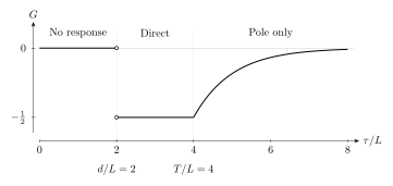
For $\lambda L=2$, $x'=L$ and $x=3L$, the exact delta-barrier kernel first arrives at $\tau=2L$. It stays at $-1/2$ until $\tau=4L$, after which the single damped-pole expression is exact. The ordinate is dimensionless; the plot is quantitative for this flat one-dimensional model, not a black-hole waveform. Values at the wavefront are interpreted distributionally.

The residue rule indeed gives $-\tfrac12e^{-\lambda(\tau-T)/2}$. Extending it backward would predict a nonzero signal before $d$ and miss the direct plateau. The full kernel contains spatial factors with the longer delay $T$, so discarding the entire lower arc is justified only after $\tau\gt T$ in this calculation. The algebraic $1/\omega^2$ decay of the barrier correction does not defeat exponential growth before that time.

For opposite-side points, $d=T$: the direct-only interval disappears and the transmitted exponential begins at the first arrival. Finally, $\lambda\to0$ at fixed $\tau$ recovers the free kernel $-\theta(\tau-d)/2$. The statement that zero frequency is removable assumed $\lambda\ne0$; the free kernel itself has a zero-frequency pole.

A convergent cut need not be the causal inverse

The delta kernel is meromorphic. To test the cut formula separately, take a different transfer function, not the same spatial wave operator:

$$F(\omega)=e^{i\omega T} \int_0^\infty\frac{e^{-\alpha\nu}}{\nu-i\omega}\,d\nu, \qquad \alpha\gt 0,\quad T\geq0.$$

Both $\alpha$ and $T$ have time units. For $\operatorname{Im}\omega\gt 0$, the integral converges absolutely. Since $1/(\nu-i\omega)$ is the transform of $\theta(\tau)e^{-\nu\tau}$, an absolutely convergent interchange of the time and $\nu$ integrals gives

$$f_{\mathrm{ret}}(\tau)= \frac{\theta(\tau-T)}{\alpha+\tau-T}.$$

The right side means the displayed quotient on $\tau\gt T$ and zero otherwise; it has no singularity at the excluded time $T-\alpha$. Its late decay is algebraic, unlike the delta barrier’s exponential.

On the downward cut, the denominator is $\nu'-\nu\mp i0$ on its east/west banks. The distributional identity $1/(z-i0)-1/(z+i0)=2\pi i\delta(z)$ therefore gives

$$\Delta F(-i\nu)=2\pi i\,e^{(T-\alpha)\nu}.$$

Our oriented cut integral becomes

$$-\frac{i}{2\pi}\int_0^\infty e^{-\nu\tau}\Delta F(-i\nu)\,d\nu =\frac{1}{\alpha+\tau-T}, \qquad \tau\gt T-\alpha.$$

For $\tau\gt T$ it is the causal answer. But in the interval $T-\alpha\lt \tau\lt T$, the integral still converges and is nonzero, whereas the causal response is exactly zero. A discarded contour contribution must cancel it there. Convergence of a cut integral does not establish the validity of the deformation with its other pieces omitted. The preceding massive-kernel example demonstrates the same issue for a spatial wave equation and a different cut.

From an impulse kernel to a source waveform

A kernel is not yet an excited waveform. For zero prehistory and

$$P\Psi=f(t)\delta(x-x'), \qquad \operatorname{supp}f\subseteq[0,t_s],$$

the delta-barrier solution is

$$\Psi(t,x)=\int_0^{t_s}G_{\mathrm{ret}}(t-s;x,x')f(s)\,ds.$$

Every source time is in the pole-only regime only when $t\gt T+t_s$. Then, with $a=\lambda/2$,

$$\Psi(t,x) =-\frac12e^{-a(t-T)} \int_0^{t_s}e^{as}f(s)\,ds, \qquad t\gt T+t_s.$$

Thus the residue’s excitation depends on the source and can vanish. For an extended source, the valid onset must cover the largest relevant source-to-observer delay as well as the source duration. Exchanging a late-time kernel expansion with source integration requires a uniform time region and an integrable bound; a pointwise estimate at one source position is insufficient.

In a black-hole application also specify the continuation sheet, convergence meaning of an infinite pole sum, cut endpoint limits, and observable projection. Prompt response, ringing, and tails are useful regime descriptions, not a universal three-stage partition. A cut can eventually dominate damped poles when its coefficient is nonzero and no growing mode intervenes. A pole list alone proves neither excitation nor completeness.

The local Hadamard direct/tail decomposition instead describes singularities within a normal neighborhood. Its tail coefficient $V(x,x')$ must not be identified pointwise with the global branch-cut term. Relating the two representations requires an overlap domain. The next chapter develops quasinormal boundary conditions and resonances; detector likelihoods and waveform inference require a model of the observation.

Exercises

1. A causal but unstable inverse. Set $\lambda=-2a$ with $a\gt 0$. Find the unstable pole, a normalized bound eigenfunction of $H=-\partial_x^2-2a\delta(x)$, and the correct Bromwich placement. Does instability destroy finite propagation?

Solution

The pole is $\omega=ia$. The normalized function

$$\psi_b(x)=\sqrt a\,e^{-a|x|}, \qquad H\psi_b=-a^2\psi_b,$$

has norm one because $2a\int_0^\infty e^{-2ax}\,dx=1$, and its derivative jump is $-2a\psi_b(0)$ as required. The wave equation $\partial_t^2\Psi+H\Psi=0$ therefore admits $e^{at}\psi_b$.

Choose $\gamma\gt a$, not a real-axis Fourier contour below the pole. The same delayed inversion, now performed above the growth bound, gives

$$G_{\mathrm{ret}} =-\frac12\theta(\tau-d) +\frac12\theta(\tau-T)\left[1-e^{a(\tau-T)}\right].$$

It still vanishes before $d$, yet grows after $T$. A growing mode is compatible with causality. The bound-mode contribution alone need not have the full kernel’s finite-propagation support; the remaining spectral contribution is necessary before the appropriate late-time regime.

2. A pole without a late waveform. Return to $\lambda=2a\gt 0$. Construct a nonzero finite-duration source whose waveform vanishes for $t\gt T+t_s$, even though the Green function still has its pole.

Solution

Take a differentiable function $h$ supported on $[0,t_s]$, with $h(0)=h(t_s)=0$, and let $f(s)=e^{-as}h'(s)$. For example, use $h(s)=s^2(t_s-s)^2$ inside the interval and zero outside. Then

$$\int_0^{t_s}e^{as}f(s)\,ds =h(t_s)-h(0)=0.$$

The late waveform is therefore exactly zero. The source can produce a nonzero direct transient; its weighted positive and negative parts cancel the pole’s excitation, not the pole of the kernel. Restricting the source to a nonnegative function would prevent this cancellation unless it vanished almost everywhere.

References

• Casals, M., and Ottewill, A. C. (2013). “Analytic investigation of the branch cut of the Green function in Schwarzschild space-time.” Physical Review D 87, 064010. DOI. Open PDF, arXiv:1210.0519v1.
• Hui, L., Kabat, D., and Wong, S. S. C. (2019). “Quasinormal modes, echoes and the causal structure of the Green’s function.” Journal of Cosmology and Astroparticle Physics 12, 020. DOI. Open PDF.
• Leaver, E. W. (1986). “Spectral decomposition of the perturbation response of the Schwarzschild geometry.” Physical Review D 34, 384–408. DOI. Open PDF, author version.