In, Up, Out, and Down Scattering Bases

In and Up specify radiation supplied by the two past boundaries; Out and Down specify radiation received at the two future boundaries. These are two bases of one two-dimensional solution space, not four independent degrees of freedom. For a massless scalar on a subextremal Kerr exterior, we derive their connection matrix, the physical scattering matrix, and the frequency factors that convert amplitudes into fluxes. A solvable interface example checks both ordinary scattering and the superradiant sign.

Required background. PDEs and Green Functions for Gravitation supplies fundamental solution bases and conserved currents.

Helpful background. Black-Hole Geometry and Mechanics fixes horizon generators and asymptotic ends; Formulations of General Relativity supplies the separated radial equations; Events, Intervals, and Minkowski Geometry fixes causal wave orientation; Black-Hole Perturbation Theory supplies the physical master variables.

Scalar radial waves and causal endpoints

Take the exterior $r>r_+$ of a fixed Kerr black hole, with physical mass $M$, spin length $a=J/M$, and $|a|\lt GM$. Write

$$\begin{gathered} \Delta=r^2-2GMr+a^2,\qquad h=r^2+a^2,\\ r_+=GM+\sqrt{G^2M^2-a^2},\qquad \frac{dx}{dr}=\frac{h}{\Delta},\qquad \Omega_H=\frac{a}{r_+^2+a^2}. \end{gathered}$$

The tortoise coordinate $x$ increases from the horizon to infinity. For a separated solution of $\Box_g\Phi=0$, use

$$\Phi=e^{-i\omega t+im\phi}S_{\ell m}(\theta;a\omega) \frac{R(x)}{\sqrt h}.$$

Here $\omega>0$ is real, $\ell\geq |m|$, and the scalar spheroidal harmonic is regular at both poles. Let $A_{0\ell m}$ be the angular eigenvalue in the angular Teukolsky equation, and set $\lambda=A_{0\ell m}+a^2\omega^2-2am\omega$. This field rescaling removes the first radial derivative:

$$\begin{aligned} R''+Q R&=0,\\ Q&=\left(\omega-\frac{am}{h}\right)^2-\frac{\lambda\Delta}{h^2} -\frac{2(GMr-a^2)\Delta}{h^3} -\frac{3a^2\Delta^2}{h^4}. \end{aligned}$$

Primes hereafter mean $d/dx$. One obtains this equation by substituting $U=R/\sqrt h$ into $\partial_r(\Delta\partial_r U)+(K^2/\Delta-\lambda)U=0$, where $K=h\omega-am$, and using $\partial_x=(\Delta/h)\partial_r$. Thus $Q$ is real and has dimension inverse length squared. At $a=0$ it reduces to $\omega^2-f[\ell(\ell+1)/r^2+2GM/r^3]$, with $f=1-2GM/r$. The radial rescaling and potential agree with Ottewill and Winstanley 2000, § II, pp. 3–4, Eqs. (2.2), (2.6)–(2.10), PDF; their potential is $-Q$ and their geometrized mass is $GM$.

At infinity $Q\to\omega^2$; at the horizon $Q\to k_H^2$, where $k_H=\omega-m\Omega_H$. Exclude $\omega=0$ and $k_H=0$ throughout the traveling-wave construction. The four endpoint components are:

Component	Radial factor	Causal role
Infinity input	$e^{-i\omega x}$	Arrives from past null infinity
Infinity output	$e^{+i\omega x}$	Reaches future null infinity
Horizon input	$e^{+ik_Hx}$	Emerges from the past horizon
Horizon output	$e^{-ik_Hx}$	Enters the future horizon

The last identification does not change when $k_H\lt0$. In ingoing Kerr coordinates $v=t+x$ and $\widetilde\phi=\phi+\int a\,dr/\Delta$, the complete future-horizon phase becomes $e^{-i\omega v+im\widetilde\phi}$ times a regular radial factor. Regularity, not the sign of $k_H$, selects that endpoint. In Schwarzschild, $e^{-i\omega x}$ is inward-propagating at both ends, but past-infinity incidence and future-horizon absorption are different boundary roles. The past-horizon channel belongs to the eternal exterior’s scattering problem; it does not assert that a collapsing star emits from a physical past horizon.

The In and Up basis

Normalize the In solution to unit amplitude from past null infinity:

$$R^{\mathrm{in}}\sim \begin{cases} T_{\mathrm{in}}e^{-ik_Hx}, & x\to-\infty,\\ e^{-i\omega x}+R_{\mathrm{in}}e^{+i\omega x}, & x\to+\infty. \end{cases}$$

There is no component emerging from the past horizon. Normalize the Up solution to unit emergence from the past horizon:

$$R^{\mathrm{up}}\sim \begin{cases} e^{+ik_Hx}+R_{\mathrm{up}}e^{-ik_Hx}, & x\to-\infty,\\ T_{\mathrm{up}}e^{+i\omega x}, & x\to+\infty. \end{cases}$$

There is no input from past null infinity. Superscripts label solutions; subscripts on $R_{\mathrm{in}}$ and $R_{\mathrm{up}}$ label reflection coefficients. These are the source’s $R^+$ and $R^-$, respectively (Ottewill and Winstanley 2000, § II, p. 4, Eq. (2.11), PDF).

Assume these finite incident normalizations exist. For the endpoint-normalized solutions $u_L\sim e^{-ik_Hx}$ at the horizon and $u_R\sim e^{i\omega x}$ at infinity, this requires a nonzero Wronskian. Indeed, writing $u_L=A_{\mathrm{inc}}e^{-i\omega x} +A_{\mathrm{ref}}e^{i\omega x}$ at infinity gives $W[u_L,u_R]=2i\omega A_{\mathrm{inc}}$. Then $R^{\mathrm{in}}=u_L/A_{\mathrm{inc}}$. This connects the present normalization to mode Green functions. It also identifies what would fail if the incident coefficient vanished.

The Out and Down basis

Because $Q$ is real at fixed $(\omega,\ell,m)$, conjugating the radial function gives another solution of the same radial equation. Define

$$R^{\mathrm{out}}=(R^{\mathrm{in}})^*, \qquad R^{\mathrm{down}}=(R^{\mathrm{up}})^*.$$

The endpoint terms fix the causal interpretation without relying on the name. For Out, the unit $e^{+i\omega x}$ term travels from the interaction region to future null infinity; the $R_{\mathrm{in}}^*e^{-i\omega x}$ term is supplied from past null infinity, while $T_{\mathrm{in}}^*e^{+ik_Hx}$ emerges from the past horizon. For Down, the unit $e^{-ik_Hx}$ term enters the future horizon; the $R_{\mathrm{up}}^*e^{+ik_Hx}$ and $T_{\mathrm{up}}^*e^{-i\omega x}$ terms are supplied from the past horizon and past null infinity, respectively. Thus $\{R^{\mathrm{out}},R^{\mathrm{down}}\}$ is normalized by one unit future output at infinity or at the horizon.

Conjugating the complete spacetime mode instead flips both $(\omega,m)$ to $(-\omega,-m)$, with the corresponding angular phase convention. The future endpoint interpretation is also explicit in Ottewill and Winstanley 2000, § III B, pp. 7–8, Eqs. (3.8), (3.10), PDF; here we retain classical amplitudes, not quantum mode normalizations. In the diagram, inspect the bold unit arrows: In and Up fix one past input; Out and Down fix one future output.

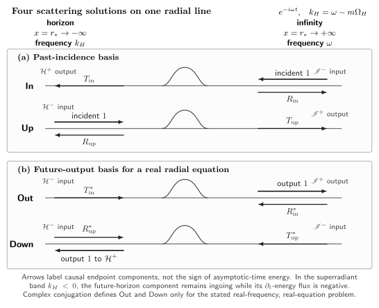
The four real-frequency radial solutions on a schematic tortoise-coordinate line. The horizon waves use $k_H=\omega-m\Omega_H$ and the infinity waves use $\omega$. Arrow direction labels the causal endpoint component, not the sign of $\partial_t$-energy flux: in the superradiant band the future-horizon wave is still ingoing even though that energy flux is negative. The barrier shape and distances are not to scale, and the conjugation relation applies only to the stated real radial equation.

Scattering matrix versus basis connection

Let $a_\infty,a_H$ be the two past-input amplitudes and $b_\infty,b_H$ the two future-output amplitudes. A general solution has

$$\begin{aligned} R&=a_\infty R^{\mathrm{in}}+a_H R^{\mathrm{up}}\\ &=b_\infty R^{\mathrm{out}}+b_H R^{\mathrm{down}}. \end{aligned}$$

Reading the output coefficients of In and Up gives the physical scattering map:

$$\boldsymbol b=S\boldsymbol a,\qquad S=\begin{pmatrix} R_{\mathrm{in}}&T_{\mathrm{up}}\\ T_{\mathrm{in}}&R_{\mathrm{up}} \end{pmatrix}, \qquad \boldsymbol a=\binom{a_\infty}{a_H},\quad \boldsymbol b=\binom{b_\infty}{b_H}.$$

By contrast, the relation between columns of basis functions is

$$\begin{pmatrix}R^{\mathrm{in}}\\R^{\mathrm{up}}\end{pmatrix} =C \begin{pmatrix}R^{\mathrm{out}}\\R^{\mathrm{down}}\end{pmatrix}.$$

Its first row is $R^{\mathrm{in}}=R_{\mathrm{in}}R^{\mathrm{out}} +T_{\mathrm{in}}R^{\mathrm{down}}$: the two coefficients reproduce the two outputs. Consequently

$$C=S^{\mathsf T} =\begin{pmatrix} R_{\mathrm{in}}&T_{\mathrm{in}}\\ T_{\mathrm{up}}&R_{\mathrm{up}} \end{pmatrix}.$$

The transpose comes from the distinction between a list of functions and the coefficients multiplying that list. These matrices are not the transfer matrix that relates two traveling-wave coefficients at one spatial end to the two at the other.

Use $W[u,v]=uv'-vu'$. If $u=c_1v_1+c_2v_2$, then

$$c_1=\frac{W[u,v_2]}{W[v_1,v_2]}, \qquad c_2=\frac{W[v_1,u]}{W[v_1,v_2]}.$$

The radial equation makes $W'=0$. Evaluating $W[R^{\mathrm{in}},R^{\mathrm{up}}]$ at the two ends gives

$$W[R^{\mathrm{in}},R^{\mathrm{up}}] =2i\omega T_{\mathrm{up}}=2ik_H T_{\mathrm{in}}.$$

Thus amplitude reciprocity includes a frequency factor: $\omega T_{\mathrm{up}}=k_HT_{\mathrm{in}}$. Since the future pair is the conjugate of the past pair,

$$\det C=\frac{W[R^{\mathrm{in}},R^{\mathrm{up}}]} {W[R^{\mathrm{out}},R^{\mathrm{down}}]} =-\frac{T_{\mathrm{up}}}{T_{\mathrm{up}}^*}, \qquad |\det C|=1.$$

This uses a nondegenerate pair, hence $T_{\mathrm{up}}\ne0$. The determinant is a phase, not necessarily $1$.

Conserved current and signed flux normalization

For this real radial equation,

$$j[R]=\frac{R^*R'-RR'^*}{2i},\qquad j'=\frac{R^*R''-RR''^*}{2i}=0.$$

For $R=Ae^{-ikx}+Be^{ikx}$, the cross terms cancel and $j=k(|B|^2-|A|^2)$. Evaluating the current of each incident solution, and the mixed Wronskian $W[(R^{\mathrm{in}})^*,R^{\mathrm{up}}]$, gives

$$\begin{aligned} \omega(1-|R_{\mathrm{in}}|^2)&=k_H|T_{\mathrm{in}}|^2,\\ k_H(1-|R_{\mathrm{up}}|^2)&=\omega|T_{\mathrm{up}}|^2,\\ \omega R_{\mathrm{in}}^*T_{\mathrm{up}} +k_HT_{\mathrm{in}}^*R_{\mathrm{up}}&=0. \end{aligned}$$

Together with transmission reciprocity, these are the four relations in Ottewill and Winstanley 2000, § II, p. 4, Eq. (2.12), PDF. The mixed identity matters: checking In and Up separately does not check the interference of arbitrary coherent inputs.

For the general solution, the endpoint currents are $j_\infty=\omega(|b_\infty|^2-|a_\infty|^2)$ and $j_H=k_H(|a_H|^2-|b_H|^2)$. Equating them yields

$$\boldsymbol b^\dagger D\boldsymbol b =\boldsymbol a^\dagger D\boldsymbol a,\qquad S^\dagger D S=D,\qquad D=\operatorname{diag}(\omega,k_H).$$

At fixed positive $\omega$, the scalar $\partial_t$-energy current is a common positive multiple of $\omega j$. In particular, the energy absorbed by the hole from an In wave is proportional to $\omega k_H|T_{\mathrm{in}}|^2$. It is negative when $k_H\lt0$: the outgoing energy at infinity exceeds the incident energy. The causal horizon wave is still the future-ingoing one.

Unit incident amplitude therefore is not unit flux. Define amplitudes measured in units of absolute current by

$$\begin{gathered} N=\operatorname{diag}(\sqrt\omega,\sqrt{|k_H|}),\qquad \widehat{\boldsymbol a}=N\boldsymbol a,\quad \widehat{\boldsymbol b}=N\boldsymbol b,\\ \widehat S=N S N^{-1},\qquad \mathcal J=\operatorname{diag}(1,\operatorname{sgn}k_H). \end{gathered}$$

Then

$$\widehat S^\dagger\mathcal J\widehat S=\mathcal J,\qquad \mathcal J\widehat S=\widehat S^{\mathsf T}\mathcal J.$$

For $k_H>0$, $\widehat S$ is unitary and symmetric in this phase convention. For $k_H\lt0$, it preserves an indefinite form instead; replacing $k_H$ by $|k_H|$ in $D$ would erase superradiance. Equivalently, divide In and Out by $\sqrt\omega$, and Up and Down by $\sqrt{|k_H|}$, to obtain unit absolute-current basis functions. The extra common factor $\sqrt\omega$ converts current to energy normalization at fixed frequency.

An exactly solvable interface check

To test the algebra without a numerical Kerr solver, replace the radial coefficient by a step and a delta barrier:

$$R''+\bigl[k^2\Theta(-x)+\omega^2\Theta(x) -\gamma\delta(x)\bigr]R=0, \qquad k=k_H.$$

Here $\omega>0$, $k\ne0$, and $\gamma$ is real; all three have dimension inverse length. This is a prescribed real radial matching model, not a Kerr potential or a claim about its mode stability. Retain the same causal endpoint labels. Distributional matching requires

$$[R]_0=0,\qquad [R']_0=\gamma R(0), \qquad [F]_0=F(0^+)-F(0^-).$$

For In these conditions read $T_{\mathrm{in}}=1+R_{\mathrm{in}}$ and $i\omega(R_{\mathrm{in}}-1)+ikT_{\mathrm{in}} =\gamma T_{\mathrm{in}}$. Solving this pair, and the corresponding Up pair, gives

$$\begin{aligned} R_{\mathrm{in}}&=\frac{\omega-k-i\gamma}{\omega+k+i\gamma}, &T_{\mathrm{in}}&=\frac{2\omega}{\omega+k+i\gamma},\\ R_{\mathrm{up}}&=\frac{k-\omega-i\gamma}{\omega+k+i\gamma}, &T_{\mathrm{up}}&=\frac{2k}{\omega+k+i\gamma}. \end{aligned}$$

The common denominator must be nonzero. For any length $L>0$, two exact checks with $\omega L=2$ and $\gamma L=1$ are:

$kL$	$R_{\mathrm{in}}$	$T_{\mathrm{in}}$	Reflected fraction	Absorbed fraction
$1$	$(1-2i)/5$	$(6-2i)/5$	$1/5$	$4/5$
$-1$	$1-2i$	$2-2i$	$5$	$-4$

The last two columns are $|R_{\mathrm{in}}|^2$ and $(k/\omega)|T_{\mathrm{in}}|^2$, and sum to one in each row. For $\gamma=0$ and $k=\omega$, both transmissions are $1$ and both reflections vanish: with the infinity/horizon channel order, $S$ exchanges the channels rather than being the identity. For $\gamma=0$ and $k=-\omega$, the denominator vanishes. An outgoing-only solution then exists in this model, so the unit-incidence construction is singular. This exception is not evidence for a real-frequency Kerr mode.

Limits of the traveling-wave construction

At $k_H=0$, the horizon exponentials coincide and unit flux normalization is singular. A regular threshold basis or a controlled limit is needed. The same warning applies at $\omega=0$. For a massive field of mass $\mu$, the infinity wavenumber becomes $q_\infty=\sqrt{\omega^2-\mu^2}$; its threshold and below-threshold exponentials require new endpoint conditions and an explicit branch choice.

For complex frequency, conjugation generally does not give a second solution at the same spectral parameter. An absorbing medium or a complex effective radial potential also invalidates this simple current argument. Spin-weighted Teukolsky functions have different radial powers and flux conversions; use their actual equations and identities, not these bare scalar coefficients. See physical Teukolsky radial solutions and reflection, transmission, and absorption.

Exercises

Recover a mixed identity. Evaluate $W[(R^{\mathrm{in}})^*,R^{\mathrm{up}}]$ at both ends. Why do the two separate incident flux balances not replace this check?

Solution

At infinity only the pairing of $R_{\mathrm{in}}^*e^{-i\omega x}$ with $T_{\mathrm{up}}e^{i\omega x}$ survives. At the horizon only the pairing of $T_{\mathrm{in}}^*e^{ik_Hx}$ with $R_{\mathrm{up}}e^{-ik_Hx}$ survives. Therefore

$$2i\omega R_{\mathrm{in}}^*T_{\mathrm{up}} =-2ik_HT_{\mathrm{in}}^*R_{\mathrm{up}}.$$

The separate flux balances give the diagonal entries of $S^\dagger D S$; this Wronskian gives its off-diagonal entry and controls interference. Taking $k_H=\omega$ removes the transmission frequency factor but does not generally make the two complex reflection amplitudes equal.

Move the tortoise origin. Replace $x$ by $y=x+c$, with real constant $c$, and reimpose unit incident amplitudes using exponentials in $y$. Find the changes in all four coefficients. Which fluxes change?

Solution

Substitute $x=y-c$ into each endpoint formula. Multiply the old In solution by $e^{-i\omega c}$ and the old Up solution by $e^{ik_Hc}$ to restore their unit inputs. The new coefficients are

$$\begin{aligned} R_{\mathrm{in}}^{\mathrm{new}}&=e^{-2i\omega c}R_{\mathrm{in}},& R_{\mathrm{up}}^{\mathrm{new}}&=e^{2ik_Hc}R_{\mathrm{up}},\\ T_{\mathrm{in}}^{\mathrm{new}}&=e^{i(k_H-\omega)c}T_{\mathrm{in}},& T_{\mathrm{up}}^{\mathrm{new}}&=e^{i(k_H-\omega)c}T_{\mathrm{up}}. \end{aligned}$$

All four magnitudes, hence the single-channel flux fractions, are unchanged. Transmission reciprocity survives because both transmissions acquire the same phase. Scattering phases require a declared coordinate and endpoint phase convention even when flux ratios do not.

References

• Ottewill, A. C., and Winstanley, E. (2000). “The renormalized stress tensor in Kerr space-time: general results.” Physical Review D 62, 084018. DOI. Open PDF, arXiv:gr-qc/0004022v2; cited page numbers are this version’s printed labels.