Retarded Green Functions on Black-Hole Exteriors

A retarded Green function tells us how a localized disturbance influences later observations. For a specified wave operator on a globally hyperbolic black-hole exterior, zero past data select a unique causal response. A timelike outer boundary changes the problem: its boundary condition must also be specified. We first establish this distinction, then derive the normalized local light-cone and interior response for a scalar field. A local formula is not a substitute for the global propagator.

Required background. PDEs and Green Functions for Gravitation supplies distributions, normally hyperbolic operators, and the Cauchy problem.

Helpful background. Black-Hole Geometry and Mechanics identifies the exterior and its boundaries; Formulations of General Relativity supplies gauge and constraint propagation; Events, Intervals, and Minkowski Geometry supplies causal orientation; Black-Hole Perturbation Theory introduces the master fields.

The causal inverse and its source normalization

Let $M$ be a smooth, time-oriented Lorentzian spacetime without boundary and consider the scalar operator

$$P=\Box_g-\mathcal U(x), \qquad \mathcal U\in C^\infty(M,\mathbb R).$$

The highest-derivative part is the metric wave operator, so $P$ is normally hyperbolic. The smooth potential $\mathcal U$ does not change its light cones. For example, a massive curvature-coupled scalar has $\mathcal U=\mu^2+\xi R$, where $\mu$ has inverse-length units, $\xi$ is a dimensionless constant, and $R$ is the Ricci scalar.

Write $G_{\mathrm{ret}}(x,x')$ for the distribution kernel with observation point $x$ and source point $x'$. Our normalization is

$$P_xG_{\mathrm{ret}}(x,x')=\delta_g(x,x'), \qquad \operatorname{supp}G_{\mathrm{ret}}(\,\cdot\,,x') \subseteq J^+(x').$$

Here $J^+(x')$ includes all points reachable from $x'$ by future-directed causal curves. The invariant delta is defined by $\int_M\delta_g(x,x')f(x)\,dV_g(x)=f(x')$. For a smooth compactly supported source $f$, the corresponding operator is

$$(G_{\mathrm{ret}}f)(x) =\int_M G_{\mathrm{ret}}(x,x')f(x')\,dV_g(x').$$

The field is zero outside the causal future of the source. This is a spacetime support statement, not a choice of quantum state. A small imaginary frequency displacement represents it only after the transform convention and sufficient growth bounds have been established.

The Cauchy construction

Theorem. Assume in addition that $M$ is globally hyperbolic. There is a unique continuous linear retarded Green operator from $C_c^\infty(M)$ to $C^\infty(M)$ such that

$$P G_{\mathrm{ret}}f=f, \qquad G_{\mathrm{ret}}P f=f, \qquad \operatorname{supp}(G_{\mathrm{ret}}f) \subseteq J^+(\operatorname{supp}f).$$

There is an analogous advanced operator with past support. Global hyperbolicity equivalently means that $M$ admits a Cauchy surface, meeting every inextendible causal curve exactly once; no unprescribed timelike boundary can inject data. The theorem does not require a positive conserved energy. Causal well-posedness and late-time stability are different assertions.

The input is the smooth Cauchy theorem: on such an $M$, for a smooth spacelike Cauchy surface $\Sigma$ with future unit normal $n$, any compact smooth source $f$ and compact smooth data $(u_0,u_1)$ on $\Sigma$ determine one smooth solution of

$$Pu=f,\qquad u|_\Sigma=u_0,\qquad n^a\nabla_a u|_\Sigma=u_1.$$

It depends continuously on the data and has finite propagation speed; its support is contained in the causal set generated by the source and initial-data supports. The energy-estimate and patching proof of this input is in Bär, Ginoux, and Pfäffle 2007, Theorems 3.2.11–3.2.12, pp. 85–86.

Construction. Choose a Cauchy surface earlier than the compact support of $f$ and solve with zero data there. Past uniqueness makes the field zero before the source; future domain of dependence gives the stated retarded support. A different sufficiently early surface gives the same solution: both fields are zero on an earlier common surface and solve the same inhomogeneous equation. Thus $G_{\mathrm{ret}}f$ is well defined and linear, and $P G_{\mathrm{ret}}f=f$.

For the other inverse identity, the compact smooth function $f$ itself solves $Pu=Pf$ and has zero data on a surface before its support. Uniqueness therefore gives $G_{\mathrm{ret}}Pf=f$. Finally, if two retarded operators exist, apply their difference to an arbitrary compact smooth source. The resulting smooth field is homogeneous with zero earlier Cauchy data, hence vanishes. Equality for every test source proves equality of their distribution kernels; we have not applied a smooth theorem directly to an unsmeared point singularity.

These are the Green-operator identities of Bär, Ginoux, and Pfäffle 2007, Definition 3.4.1 and Corollary 3.4.3, pp. 88–89. Two source conventions require translation. Their principal wave term is $-g^{ab}\partial_a\partial_b$, opposite to ours: apply their theorem to $-P$ and negate its inverse. Their “advanced” operator has future support and is called retarded here Bär, Ginoux, and Pfäffle 2007, § 1.5, pp. 33–34, and Definition 3.4.1, pp. 88–89.

Horizons, outer boundaries, and reflected arrivals

A horizon is not a timelike wall

For the massless Schwarzschild master equation, the separated retarded construction selects radial endpoint phases

$$e^{-i\omega r_*}\quad\text{at the future horizon}, \qquad e^{+i\omega r_*}\quad\text{at infinity}.$$

Together with $e^{-i\omega t}$, the first depends on the regular advanced time $v=t+r_*$, and the second on outgoing retarded time $u=t-r_*$. They implement the causal response with no added incoming homogeneous radiation from the past endpoints; they are not signals supplied from the future. Mode Green Functions and Wronskians derives this frequency representation.

Do not transfer these phases unchanged to every stationary black hole. For a separated Kerr scalar mode, the horizon frequency is $k_H=\omega-m\Omega_H$, where $m$ is its azimuthal number and $\Omega_H$ the horizon angular velocity. A massive asymptotic field uses a momentum $\sqrt{\omega^2-\mu^2}$ on a specified continued sheet. Other master variables can carry additional radial prefactors. Stationarity alone does not guarantee separability.

A timelike AdS conformal boundary or an artificial worldtube instead requires a declared initial-boundary value problem. Boundary conditions do not make a non-globally-hyperbolic spacetime globally hyperbolic; they specify its dynamics. Their admissibility and uniqueness must be proved. For a concrete framework using positive self-adjoint extensions in static AdS, see Ishibashi and Wald 2004, § 1, pp. 2–3. This is not a theorem that every Robin, mixed, or transparent condition works for every rotating AdS black hole.

Dirichlet and Neumann wall conditions

The missing-boundary-condition issue is already visible in flat $1+1$ dimensions. On $x\gt0$, take $P=-\partial_t^2+\partial_x^2$, source position $x'\gt0$, elapsed time $\tau=t-t'$, and zero past data. The image construction gives

$$\begin{aligned} G_D(\tau,x,x') &=-\frac12\left[ \Theta(\tau-|x-x'|)-\Theta(\tau-x-x')\right],\\ G_N(\tau,x,x') &=-\frac12\left[ \Theta(\tau-|x-x'|)+\Theta(\tau-x-x')\right]. \end{aligned}$$

Both have the unit interior source $P G=\delta(\tau)\delta(x-x')$. The image is at $-x'$, outside the domain, so it adds no interior source. Direct substitution at the wall gives $G_D|_{x=0}=0$ and $\partial_xG_N|_{x=0}=0$: these are homogeneous Dirichlet and Neumann conditions, respectively.

Because $x+x'\gt|x-x'|$, the reflected contribution starts later than the direct one, and both kernels have retarded support. Yet

$$G_N-G_D=-\Theta(\tau-x-x').$$

The difference solves the homogeneous equation in the open interior but has different wall data. This is a counterexample to uniqueness with an unspecified boundary, not to uniqueness for either fixed wall problem.

In the diagram, follow the direct ray and then the two legs of the reflected ray. The source reaches the wall at $\tau=2L$, but the observer does not receive that reflected influence until $\tau=6L$.

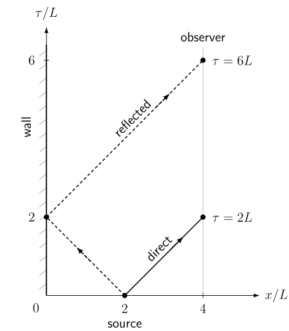
Direct and reflected null arrivals for the flat half-line wave equation, with source $x'=2L$, observer $x=4L$, and $L\gt0$. Equal coordinate scales make the ray slopes exact. The ray diagram is a schematic of arrival paths, not a plot of field amplitude or a black-hole horizon.

The same relationship is available without the figure:

Observer time	Arrival information	$G_D$	$G_N$
$\tau\lt2L$	Neither signal has arrived	$0$	$0$
$2L\lt\tau\lt6L$	Direct response only	$-1/2$	$-1/2$
$\tau\gt6L$	Direct and reflected responses	$0$	$-1$

These are dimensionless impulse-kernel values in $1+1$ dimensions, away from the wavefronts. The value assigned to a step function exactly at its front does not affect its distribution. The nonzero interior response of this flat example is not curvature scattering.

Local Hadamard form with a fixed normalization

Now work in four spacetime dimensions with $P=\Box_g-\mu^2-\xi R$. Restrict both points to a sufficiently small causally convex normal neighborhood: the relevant causal curves remain inside it, and a unique geodesic connects the points. Synge’s world function $\sigma(x,x')$ is half the signed squared geodesic distance, negative for timelike separation. The locally retarded kernel is

$$G_{\mathrm{ret}}(x,x') =-\frac{\Theta_+(x,x')}{4\pi} \left[U(x,x')\delta(\sigma) +V(x,x')\Theta(-\sigma)\right].$$

$\Theta_+$ restricts the distributions to the future of $x'$. $U$ and $V$ are smooth biscalars, meaning scalar functions of two points. The delta term carries the direct light-cone singularity; the second term describes the smooth coefficient of an interior response. $U$ is dimensionless and $V$ has inverse-length-squared units.

The coefficient $-1/(4\pi)$ is fixed by $PG=+\delta_g$, not optional. In massless four-dimensional Minkowski spacetime, with $r=|\mathbf x-\mathbf x'|$ and $\tau=t-t'$,

$$G_{\mathrm{ret}}^{\mathrm{flat},\,\mu=0} =-\frac{\delta(\tau-r)}{4\pi r}.$$

This expression is understood distributionally at the source. Its minus sign accompanies the leading term $-\partial_t^2$. The convention in Poisson, Pound, and Vega 2011, §§ 14.1–14.2, pp. 83–85, Eqs. (14.3)–(14.14), PDF instead has $PG=-4\pi\delta_g$; multiplication by $-1/(4\pi)$ translates their kernel. Their displayed curved construction is massless. We include the $\mu^2$ term by the following distributional calculation.

Transport on the cone and evolution inside it

Write $\sigma^a=\nabla^a\sigma$ and use brackets for coincidence, $[F]=F(x',x')$. The identities

$$\sigma^a\sigma_a=2\sigma,\qquad \sigma\delta'(\sigma)=-\delta(\sigma),\qquad \sigma\delta''(\sigma)=-2\delta'(\sigma)$$

reduce the terms obtained by applying $P$ to the Hadamard form. Cancellation of the $\delta'(\sigma)$ coefficient requires

$$2\sigma^a\nabla_a U+(\Box_g\sigma-4)U=0, \qquad [U]=1.$$

The solution is $U=\Delta_{\mathrm{VVM}}^{1/2}$. The van Vleck–Morette determinant $\Delta_{\mathrm{VVM}}$ measures geodesic focusing; equivalently, it is specified here by $\sigma^a\nabla_a\log\Delta_{\mathrm{VVM}}=4-\Box_g\sigma$ and coincidence value one. This is not the Kerr radial function $\Delta$.

The coefficient of $\delta(\sigma)$ then gives the cone data for $V$, while the interior coefficient gives its wave equation:

$$\begin{aligned} 2\sigma^a\nabla_a V+(\Box_g\sigma-2)V&=PU &&\text{on }\sigma=0,\\ PV&=0 &&\text{inside the cone}. \end{aligned}$$

Thus transport along the null generators determines the cone data; a characteristic wave problem determines the interior tail. Transport along geodesics alone is not the whole construction.

At coincidence, $[\sigma^a]=0$, $[\Box_g\sigma]=4$, and $[\Box_gU]=R(x')/6$. Consequently

$$[V]=-\frac12\left[\mu^2+ \left(\xi-\frac16\right)R(x')\right].$$

The curvature identity and massless coincidence value are explicitly derived in Poisson, Pound, and Vega 2011, p. 85, Eqs. (14.10)–(14.14), PDF. The added $-\mu^2/2$ follows directly from $PU$ above.

A massive flat-space check

For flat spacetime, let $q=\sqrt{-2\sigma}$ in the timelike interior. The exact smooth coefficient is

$$U=1,\qquad V=-\frac{\mu J_1(\mu q)}{q} =-\frac{\mu^2}{2}+\frac{\mu^4q^2}{16}+O(q^4).$$

$J_1$ is the Bessel function of the first kind. It solves the interior equation and has the required cone limit Poisson, Pound, and Vega 2011, § 12.4, p. 78, Eq. (12.13), PDF. The overall negative factor in $G_{\mathrm{ret}}$ makes its leading massive interior term positive. As $\mu\to0$, this interior term vanishes and the massless direct kernel remains.

This example separates two ideas often conflated: a tail means interior support, whereas curvature scattering is one possible cause. A mass already produces interior support in flat four-dimensional spacetime. Conversely, $[V]=0$ at one point does not establish the absence of a tail. In particular, the vanishing Ricci scalar of Schwarzschild does not eliminate its global scattering response.

The local existence statement uses a sufficiently small causal domain Bär, Ginoux, and Pfäffle 2007, Proposition 2.4.11 and Corollary 2.4.12, p. 56. Its formal Hadamard series is an asymptotic construction with controlled remainders, not an automatically convergent infinite series Bär, Ginoux, and Pfäffle 2007, Theorem 2.5.2, pp. 59–61. Beyond caustics or returning null rays, one cannot simply retain the same single-geodesic expression as the global propagator. Mode sums and frequency integrals require their own convergence and contour arguments.

Green’s identity, reciprocity, and source compatibility

For our real scalar potential, $P$ is formally self-adjoint. Set $u=G_{\mathrm{ret}}f$ and $v=G_{\mathrm{adv}}h$ for compact smooth $f,h$. The current

$$j^a=\overline v\,\nabla^a u-u\nabla^a\overline v$$

obeys

$$\nabla_a j^a=\overline v\,Pu-u\,\overline{Pv} =\overline v\,f-u\,\overline h.$$

Its support lies in $J^+(\operatorname{supp}f)\cap J^-(\operatorname{supp}h)$, which is compact by global hyperbolicity. Integrating its divergence therefore gives no boundary contribution. With $\langle h,u\rangle=\int_M\overline h\,u\,dV_g$, this proves

$$\langle h,G_{\mathrm{ret}}f\rangle =\langle G_{\mathrm{adv}}h,f\rangle, \qquad G_{\mathrm{ret}}^\dagger=G_{\mathrm{adv}}.$$

Equivalently, as distribution kernels,

$$G_{\mathrm{ret}}(x,x') =\overline{G_{\mathrm{adv}}(x',x)}.$$

This exchanges source and observation and retarded and advanced conditions; it does not make a retarded kernel symmetric in its arguments. With a timelike boundary, this proof requires adjoint-compatible boundary conditions that cancel the boundary concomitant $n_a j^a$ (as the real homogeneous Dirichlet or Neumann conditions do). Causal support alone does not cancel an arbitrary boundary flux.

For gravitational perturbations, one must additionally use a gauge-invariant master variable or a gauge-fixed hyperbolic system with propagating constraints. On a vacuum background, for example, the linearized Bianchi identity forces the linearized stress-energy source to be conserved. On a matter background the coupled linearized matter equations and identities must be included. A componentwise gauge-fixed inverse applied to incompatible sources need not solve the full constrained system. Retarded support cannot repair that incompatibility.

The result here is a classical causal inverse for its stated domain. It does not select a quantum vacuum or prove that quasinormal modes alone reconstruct every response. Continue with Mode Green Functions and Wronskians to connect this spacetime object to a radial source jump.

Exercises

Check the wall and the source. Verify the Dirichlet trace and Neumann normal derivative of the half-line kernels. Show that their source normalization is positive and find the first time when an observer can distinguish them.

Solution

At $x=0$, the two step arguments are both $\tau-x'$, so the Dirichlet terms cancel. For $0\lt x\lt x'$, the direct argument is $\tau-x'+x$. Differentiating the sum in $G_N$ gives opposite delta terms at the wall, so $\partial_xG_N=0$ there.

The direct term is continuous across $x=x'$. Its spatial derivative has jump $\delta(\tau)$; the image term is smooth across this spatial interface as a time distribution. Hence the second spatial derivative contributes $+\delta(\tau)\delta(x-x')$. Away from the source each travelling step solves $P G=0$. Finally, $G_N-G_D=-\Theta(\tau-x-x')$, so the first distinguishable response is at the reflected arrival $\tau=x+x'$, not merely the wall-arrival time $\tau=x'$.

Check the local source sign. In flat four-dimensional spacetime, pair the direct kernel with a smooth spatial test function $\varphi$. Show that $G(0^+)=0$ and $\partial_\tau G(0^+)=-\delta^{(3)}$. Explain why the bounded massive tail does not change this jump.

Solution

Let $\overline\varphi(r)$ be the angular average of $\varphi$ on the sphere of radius $r$. For $\tau\gt0$, the direct shell pairs to

$$-\int_0^\infty r\,\delta(\tau-r)\, \overline\varphi(r)\,dr =-\tau\,\overline\varphi(\tau).$$

Its initial value is zero and its initial derivative is $-\varphi(0)$. The smooth massive tail is bounded near the vertex and supported in a ball of radius $\tau$, so its pairing is $O(\tau^3)$. It contributes neither initial value nor initial derivative. Extending the field by zero for $\tau\lt0$, the term $-\partial_\tau^2$ therefore supplies $+\delta(\tau)\delta^{(3)}(\mathbf x)$, as required. Reversing only the overall Green-function sign would reverse this source.

References

• Bär, Christian, Nicolas Ginoux, and Frank Pfäffle. Wave Equations on Lorentzian Manifolds and Quantization. ESI Lectures in Mathematics and Physics. Zürich: European Mathematical Society, 2007. DOI. Open PDF.
• Ishibashi, Akihiro, and Robert M. Wald. “Dynamics in Non-Globally-Hyperbolic Static Spacetimes III: Anti-de Sitter Spacetime.” Classical and Quantum Gravity 21 (2004): 2981–3014. DOI. Open PDF.
• Poisson, Eric, Adam Pound, and Ian Vega. “The Motion of Point Particles in Curved Spacetime.” Living Reviews in Relativity 14 (2011): 7. DOI. Open PDF.