Birkhoff's Theorem with a Cosmological Constant

Adding a cosmological constant preserves Birkhoff’s symmetry enhancement, but it changes two essential details. The conserved integration constant is the Misner–Sharp energy with the vacuum-volume contribution removed, and positive $\Lambda$ admits a second local solution in which every symmetry sphere has the same area: Nariai spacetime. A proof that chooses the areal radius as a coordinate too early finds Kottler but silently loses Nariai.

Required background. The Einstein Equation supplies $R_{\mu\nu}=\Lambda g_{\mu\nu}$; Killing Fields and Isometry Groups supplies the symmetry language.

Helpful background. The Riemann Curvature Tensor supports the product-curvature check; Formulations of General Relativity supplies alternative reductions.

Within this chapter. Spherical Orbit-Space Geometry defines $h$, $r$, and the Kodama direction; Areal Radius and Spherical Mass Functions defines the ordinary Misner–Sharp energy; The Vacuum Birkhoff Theorem treats the $\Lambda=0$ case in detail.

The local Einstein–Λ theorem

Let $U$ be a connected, smooth, four-dimensional, time-oriented Lorentzian region satisfying

$$R_{\mu\nu}=\Lambda g_{\mu\nu},$$

and suppose an effective local $SO(3)$ isometry action has spacelike round two-sphere orbits of area $4\pi r^2$, with $r>0$. Then every point has a neighborhood locally isometric to one of two analytic models:

1. a Kottler model, also called Schwarzschild–de Sitter, Schwarzschild, or Schwarzschild–anti-de Sitter according to the sign of $\Lambda$, with one real constant mass parameter; or
2. when $\Lambda>0$, a Nariai model, locally $\mathrm{dS}_2\times S^2$ with equal curvature radii $\Lambda^{-1/2}$.

Each model has a nonrotational local Killing field orthogonal to the symmetry spheres, but that field need not be timelike. No asymptotic condition, regular center, event horizon, mass sign, or preferred maximal extension is assumed. Smoothness matches the primary proof; no optimal low-regularity threshold is claimed here. Schleich and Witt give the branch-complete null-coordinate integration in 2010, Theorem 1 and Eqs. (4)–(12), printed pp. 3–4, Open PDF.

The branch distinction concerns behavior on a neighborhood, not the value of one derivative at one point:

Local behavior of the invariant areal radius	Branch
$r$ is not constant on the neighborhood; $dr$ may nevertheless vanish at an isolated bifurcation point	Kottler
$dr\ne0$ but $(\nabla r)^2=0$ at an ordinary or degenerate Killing-horizon point	Kottler
$dr=0$ throughout an open neighborhood	Nariai, possible only for $\Lambda>0$

This is why neither “$dr=0$ at a point” nor “$(\nabla r)^2=0$” is a branch test.

Reduced equations and the extra symmetry

On the regular-orbit region write

$$g=h_{ab}(x)\,dx^a dx^b+r(x)^2\gamma_{ij}(y)\,dy^i dy^j, \qquad q=(\nabla r)^2_h,$$

where $h$ is Lorentzian and $\gamma$ is the unit-round sphere metric. The exact warped-product Ricci blocks are

$$R^{(4)}_{ab} =R^{(h)}_{ab}-\frac{2}{r}\nabla_a\nabla_b r, \qquad R^{(4)}_{ij} =\left(1-q-r\Box_h r\right)\gamma_{ij}.$$

In two dimensions $R^{(h)}_{ab}=\tfrac12R_hh_{ab}$. The trace-free part of the quotient equation and the angular equation therefore give

$$\nabla_a\nabla_b r =\frac12(\Box_h r)h_{ab}, \qquad 1-q-r\Box_h r=\Lambda r^2,$$

while the quotient trace gives $R_h=2\Lambda+2\Box_h r/r$.

Choose an orientation on the quotient and define

$$K_a=\epsilon_a{}^b\nabla_b r.$$

Spherical kinematics already gives $K\cdot\nabla r=0$ and $K^2=-q$. The field equation supplies the missing dynamical step:

$$\nabla_{(a}K_{b)} =\epsilon_{(b}{}^c\nabla_{a)}\nabla_c r=0.$$

The lifted four-dimensional field has no angular components. Because $K(r)=0$,

$$(\mathcal L_K g)_{ij}=2rK(r)\gamma_{ij}=0,$$

and the mixed components vanish as well. Thus $K$ is a four-dimensional Killing field on the varying-radius branch. The Killing equation remains true where $K$ vanishes at an isolated bifurcation point. Its metric dual has support only on a two-dimensional quotient, so it is locally hypersurface orthogonal.

This construction belongs to the varying-radius branch. On Nariai, $dr=0$ throughout the neighborhood, so the Kodama field itself is identically zero; the nontrivial extra Killing fields instead come from the $\mathrm{dS}_2$ factor.

The conserved Kottler mass

The ordinary Misner–Sharp energy is

$$E_{\rm MS}=\frac{r}{2G}(1-q).$$

For $\Lambda\ne0$, it is not constant on a neighborhood where $r$ varies. For $\Lambda=0$ it reduces to the conserved Schwarzschild mass, while on Nariai it is constant because $r$ itself is constant. From the pure-trace Hessian,

$$\nabla_a q =2\nabla_a\nabla_b r\,\nabla^b r =(\Box_h r)\nabla_a r,$$

and hence

$$\nabla_a E_{\rm MS} =\frac{\Lambda r^2}{2G}\nabla_a r.$$

The right-hand side is exactly the change in vacuum energy inside a sphere. Subtract it before naming the constant mass. It is convenient to use the mass length $\mu=GM$:

$$\mu =\frac r2\left(1-q-\frac{\Lambda r^2}{3}\right), \qquad M=\frac{\mu}{G} =E_{\rm MS}-\frac{\Lambda r^3}{6G}.$$

Differentiation now closes on the angular equation:

$$\nabla_a\mu =\frac12 \left(1-q-r\Box_h r-\Lambda r^2\right)\nabla_a r =0.$$

The factor $1/3$ is fixed, not conventional. Replacing it by $c$ leaves $(1-3c)\Lambda r^2\nabla_a r/2$ in the mass-length gradient.

Where $r$ varies, the constant $\mu$ gives

$$q=f(r), \qquad f(r)=1-\frac{2\mu}{r}-\frac{\Lambda r^2}{3}, \qquad K^2=-f.$$

Kottler charts, horizons, and isolated critical points

The reduced equations can be integrated directly in null coordinates. Two one-sided forms are

$$ds^2=-f(r)\,dv^2+2\,dv\,dr+r^2d\Omega_2^2,$$

and

$$ds^2=-f(r)\,du^2-2\,du\,dr+r^2d\Omega_2^2.$$

Their radial-block determinant is $-1$, even at a simple or double root of $f$. Choose the quotient orientation so that the first chart has $K=\partial_v$. At $f=0$, $K$ is nonzero and null, and $dr=(0,1)$ remains a nonzero covector. A root is therefore not an open constant-radius region.

Only where $f\ne0$ may one use $dv=dt+dr/f$ to obtain

$$ds^2=-f(r)\,dt^2+\frac{dr^2}{f(r)}+r^2d\Omega_2^2.$$

This chart is static where $f>0$ and homogeneous of Kantowski–Sachs type where $f<0$. Regular coefficients obtained by transforming this diagonal chart do not by themselves prove that an arbitrary horizon-containing solution is Kottler, because the transformation is singular at $f=0$. The direct null-coordinate integration in Schleich and Witt 2010, proof of Theorem 1, printed pp. 3–4, Eqs. (4)–(12), Open PDF supplies that missing logical step.

An isolated critical point of $r$ is different again. Setting $dr=0$ at one quotient point gives

$$\nabla_a\nabla_b r =\frac{1-\Lambda r^2}{2r}h_{ab}.$$

When $1-\Lambda r^2\ne0$, this is a nondegenerate Lorentzian saddle. In the analytic Kottler extension it is the quotient point under a bifurcation sphere of a simple Killing horizon and requires a two-null chart. At the positive-$\Lambda$ double root, by contrast, the horizon-regular Kottler chart still has nonzero $dr$ and a nonzero null Killing field. Neither case is Nariai.

Analytic model overlaps also prevent the mass parameter or branch from jumping across a connected region. This is a local continuation statement, not a choice of global topology or maximal extension.

When is the Kottler Killing field timelike?

Let $\mu=GM$ and restrict to $r>0$. The first three rows below contain the central positive-$\Lambda$, positive-mass story; the remaining rows are useful sign and limiting checks. The complete elementary root classification is:

Parameters	Positive roots of $f$	Region with $f>0$
$\Lambda>0$, $\mu>0$, $0<9\Lambda\mu^2<1$	two simple roots $r_b<r_c$	$r_b<r<r_c$
$\Lambda>0$, $\mu>0$, $9\Lambda\mu^2=1$	one double root $r_0=\Lambda^{-1/2}=3\mu$	none
$\Lambda>0$, $\mu>0$, $9\Lambda\mu^2>1$	none	none
$\Lambda>0$, $\mu=0$	$r=\sqrt{3/\Lambda}$	$0<r<\sqrt{3/\Lambda}$
$\Lambda>0$, $\mu<0$	one simple root $r_c$	$0<r<r_c$
$\Lambda=0$, $\mu>0$	$r=2\mu$	$r>2\mu$
$\Lambda=0$, $\mu\le0$	none	every $r>0$
$\Lambda<0$, $\mu>0$	one simple root $r_h$	$r>r_h$
$\Lambda<0$, $\mu\le0$	none	every $r>0$

For positive $\Lambda$ and positive mass, $f$ has one positive stationary point. Writing $\mu=\Lambda r_s^3/3$ there gives

$$f(r_s)=1-\Lambda r_s^2, \qquad 9\Lambda\mu^2=(\Lambda r_s^2)^3.$$

This proves the first three rows. Equivalently, the horizon cubic $\Lambda r^3-3r+6\mu$ has discriminant $108\Lambda(1-9\Lambda\mu^2)$. The no-static-region statement is therefore a positive-mass statement; negative mass has one positive root and a static interval.

The upper panel below plots the exact dimensionless lapse in the three positive-mass de Sitter regimes. The lower panel shows why the coalescing interval must be magnified before taking a limit.

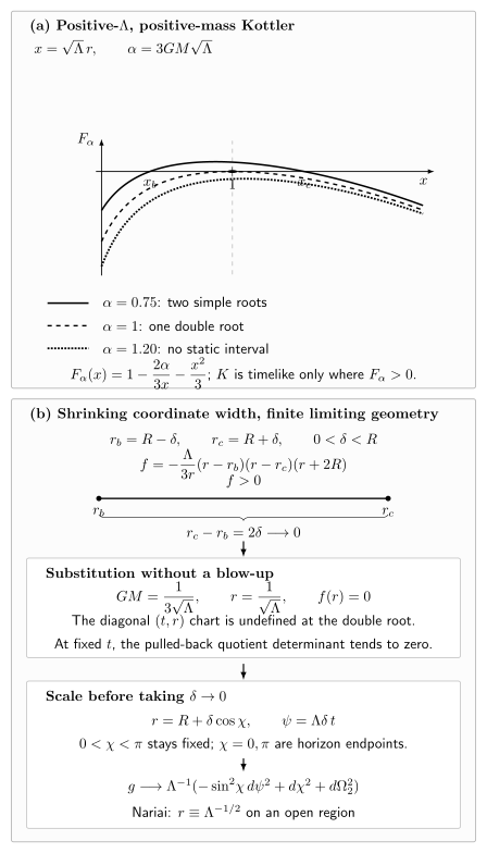
Top: the exact lapse $F_\alpha(x)=1-2\alpha/(3x)-x^2/3$ for $x=\sqrt\Lambda r$ and three representative positive values of $\alpha=3GM\sqrt\Lambda$. Solid, dashed, and dotted line styles distinguish the two-root, double-root, and no-positive-root regimes without relying on color. Bottom: the exact Kottler factorization makes the coordinate width $r_c-r_b=2\delta$ shrink, but the simultaneous scaling $r=R+\delta\cos\chi$ and $\psi=\Lambda\delta t$ retains a nondegenerate Nariai patch. The plot is quantitative; the scaling flow is schematic. The figure neither identifies extremal Kottler with Nariai nor assigns global event-horizon roles.

In the standard global positive-mass Schwarzschild–de Sitter extension, the two simple positive roots are called the black-hole and cosmological horizons. The local theorem establishes Killing-horizon roots and their causal cells; those global names require the extension. Schleich and Witt analyze all mass signs and the loss of static regions in 2010, printed pp. 4–6, Eqs. (13)–(16), Open PDF.

The open constant-radius branch

Now suppose $r=r_0>0$ throughout an open neighborhood. The metric is a direct product $h+r_0^2d\Omega_2^2$, and the Ricci equations reduce immediately to

$$R^{(h)}_{ab}=\Lambda h_{ab}, \qquad \gamma_{ij}=\Lambda r_0^2\gamma_{ij}.$$

Thus

$$\Lambda>0, \qquad r_0=\Lambda^{-1/2}, \qquad R_h=2\Lambda.$$

Every two-dimensional Lorentzian metric with scalar curvature $2\Lambda$ is locally de Sitter, so

$$(\mathcal M,g)_{\rm N} \simeq \mathrm{dS}_2(\Lambda^{-1/2}) \times S^2(\Lambda^{-1/2})$$

locally. A static product chart is

$$ds^2=\frac1\Lambda \left[-(1-y^2)d\tau^2+\frac{dy^2}{1-y^2}+d\Omega_2^2\right], \qquad -1<y<1.$$

A one-sided horizon-regular chart is

$$ds^2=(\Lambda X^2-1)du^2+2\,du\,dX +\Lambda^{-1}d\Omega_2^2.$$

Here $X$ is a coordinate on the $\mathrm{dS}_2$ factor, not the areal radius. The latter is the constant $r_0$. The vector $\partial_u$ is nonzero, Killing, timelike for $\Lambda X^2<1$, and null at $X=\pm\Lambda^{-1/2}$. This is the exceptional solution integrated directly in Schleich and Witt 2010, Eq. (10), printed pp. 3–4, Open PDF.

The product supplies sharp independent checks:

$$R=4\Lambda, \qquad R_{\mu\nu}R^{\mu\nu}=4\Lambda^2, \qquad R_{\mu\nu\rho\sigma}R^{\mu\nu\rho\sigma}=8\Lambda^2,$$

and

$$C_{\mu\nu\rho\sigma}C^{\mu\nu\rho\sigma} =\frac{16}{3}\Lambda^2.$$

Planes tangent to either factor have curvature $\Lambda$, whereas mixed planes have zero curvature. Nariai is therefore homogeneous but neither four-dimensionally constant-curvature nor conformally flat; it is Petrov type D, as summarized by Podolský and Ortaggio 2003, Eq. (38) on printed p. 7 and Table 2 on printed p. 8, Open PDF. Nariai and Bertotti–Robinson Geometries develops the product comparison further.

Same critical numbers, different geometries

For $\Lambda>0$ and $\mu>0$, a double Kottler root obeys

$$f(r_0)=f'(r_0)=0 \quad\Longrightarrow\quad r_0=\frac1{\sqrt\Lambda}, \qquad \mu_0=\frac1{3\sqrt\Lambda}.$$

Evaluating the cosmological-subtracted mass length on Nariai gives the same number:

$$\mu_{\rm N} =\frac{r_0}{2} \left(1-\frac{\Lambda r_0^2}{3}\right) =\frac1{3\sqrt\Lambda}.$$

That numerical coincidence does not identify the geometries. Nariai has $dr=0$ throughout an open set. Critical Kottler has varying areal radius and, on its degenerate horizon in a regular null chart, nonzero $dr$. Even the zeroth-order Weyl scalar does not separate the two at that sphere:

$$C^2_{\rm Kottler}=\frac{48\mu^2}{r^6} \quad\Longrightarrow\quad C^2_{\rm Kottler}(r_0)=\frac{16}{3}\Lambda^2=C^2_{\rm N}.$$

Neighborhood data do separate them. At the critical Kottler horizon,

$$d(C^2_{\rm Kottler}) =-\frac{288\mu_0^2}{r_0^7}\,dr\ne0,$$

whereas $C^2_{\rm N}$ and $r$ are constant on Nariai.

The relation between the branches is a scaled limit, not an ordinary substitution. Let two positive Kottler roots be

$$r_b=R-\delta, \qquad r_c=R+\delta, \qquad 0<\delta<R,$$

with

$$3R^2+\delta^2=\frac3\Lambda, \qquad \mu=\frac{\Lambda R(R^2-\delta^2)}{3}.$$

Then the lapse factorizes exactly as

$$f(r)=-\frac{\Lambda}{3r} (r-r_b)(r-r_c)(r+2R).$$

Before taking $\delta\to0$, introduce

$$r=R+\delta\cos\chi, \qquad \psi=\Lambda\delta\,t, \qquad 0<\chi<\pi, \qquad A_\delta(\chi)= \frac{3R+\delta\cos\chi}{3(R+\delta\cos\chi)}.$$

The open inter-root region maps to $0<\chi<\pi$; its two horizon endpoints are at $\chi=0,\pi$. On that open static patch the metric becomes exactly

$$ds^2=\frac1\Lambda \left[-A_\delta\sin^2\chi\,d\psi^2 +A_\delta^{-1}d\chi^2\right] +(R+\delta\cos\chi)^2d\Omega_2^2.$$

Its quotient determinant is $-\sin^2\chi/\Lambda^2$, independent of $\delta$ and nonzero for $0<\chi<\pi$. Its zero at either endpoint is the usual static-coordinate horizon degeneracy, not a spacetime degeneracy. Therefore

$$\delta\longrightarrow0 \quad\Longrightarrow\quad ds^2\longrightarrow\frac1\Lambda \left(-\sin^2\chi\,d\psi^2+d\chi^2+d\Omega_2^2\right),$$

the Nariai static patch. If the inverse time scaling is omitted, the quotient determinant instead tends to zero. Cardoso, Dias, and Lemos give the general near-Nariai root-and-coordinate procedure in 2004, §III.B.1, printed pp. 4–5, Eqs. (19)–(22), Open PDF. Nariai and Ultracold Limits develops the horizon-limit geometry and its charged analogues.

Scope and a discriminating adverse case

The theorem is local on a regular sphere-orbit region. It does not choose a global quotient, prove that a Killing root is an event horizon, select a maximal extension, establish mass positivity, include a regular symmetry center as a sphere orbit, or address formation and stability. Distributional shells, general matter, nonspherical perturbations, modified gravity, higher dimensions, and non-spherical orbit topology require new hypotheses.

Spherical symmetry alone remains insufficient. Replacing the constant $\mu$ by $\mu(v)$ in the ingoing metric gives cosmological Vaidya, for which

$$R_{\mu\nu}-\Lambda g_{\mu\nu} =\frac{2\dot\mu(v)}{r^2}(dv)_\mu(dv)_\nu.$$

All other residual components vanish, and $R=4\Lambda$ still holds. Thus a scalar-curvature check would miss the null flux; the full tensor equation restores Kottler only when $\dot\mu=0$.

Common pitfalls

Equating $q=0$ with $dr=0$. A nonzero null covector has zero norm. At a Kottler Killing horizon, $q=0$ while $dr$ can remain nonzero; Nariai instead has $dr=0$ throughout a neighborhood.

Calling the ordinary Misner–Sharp energy the conserved Kottler mass. With $\Lambda\ne0$ on a varying-radius branch, $E_{\rm MS}$ changes with the vacuum energy $\Lambda r^3/(6G)$. The conserved Kottler mass is the subtracted quantity; on Nariai both are constant because $r$ is constant, but they are not equal.

Reading Birkhoff as “static everywhere.” The theorem guarantees an additional local Killing field. Its norm is $-f$, so it can be timelike, null, or spacelike; critical and supercritical positive-mass de Sitter Kottler have no open static cell.

Identifying Nariai with the extremal Kottler member. They share $r_0$, $\mu_0$, and the Weyl-square value at one critical sphere, but their neighborhood geometries differ. Nariai arises from a simultaneous parameter and coordinate blow-up.

Assigning global horizon names from a local root. A root of $f$ is locally a Killing-horizon candidate in the analytic Kottler model. “Black-hole horizon,” “cosmological horizon,” and “event horizon” additionally use global extension data.

Exercises

1. Derive the conserved mass

Starting from the two reduced equations, derive $\nabla_aE_{\rm MS}$ and prove that $\mu$ is constant. For $\Lambda\ne0$ on a varying-radius neighborhood, why is the coefficient $1/3$ unique?

Solution

The pure-trace Hessian gives $\nabla_aq=(\Box_hr)\nabla_ar$. Therefore

$$\nabla_aE_{\rm MS} =\frac1{2G}(1-q-r\Box_hr)\nabla_ar =\frac{\Lambda r^2}{2G}\nabla_ar.$$

For

$$\mu_c=\frac r2(1-q-c\Lambda r^2),$$

one obtains

$$\nabla_a\mu_c =\frac12(1-3c)\Lambda r^2\nabla_ar.$$

For $\Lambda\ne0$ on a varying-radius neighborhood, $c=1/3$ is the unique coefficient that cancels the vacuum-volume term. If $\Lambda=0$, the subtraction vanishes for every $c$. The resulting $\mu=GM$ is constant in either case.

2. Classify the positive-mass de Sitter roots

Assume $\Lambda>0$ and $\mu>0$. Show that $f$ has one positive maximum and recover the two-root, double-root, and no-root criteria.

Solution

The stationary equation is

$$f'(r_s)=\frac{2\mu}{r_s^2}-\frac{2\Lambda r_s}{3}=0 \quad\Longleftrightarrow\quad \mu=\frac{\Lambda r_s^3}{3}.$$

Moreover $f''(r_s)=-2\Lambda<0$, so this is the unique positive maximum. Substitution gives

$$f(r_s)=1-\Lambda r_s^2, \qquad 9\Lambda\mu^2=(\Lambda r_s^2)^3.$$

Since $f\to-\infty$ as $r\to0^+$ and as $r\to\infty$, a positive maximum gives two simple roots, a zero maximum gives one double root, and a negative maximum gives no root. These correspond respectively to $9\Lambda\mu^2<1$, $=1$, and $>1$. The argument assumes positive mass; for $\mu<0$, $f\to+\infty$ as $r\to0^+$ and there is one positive root.

3. Verify that Nariai is Einstein but not de Sitter₄

Use the product $\mathrm{dS}_2(L)\times S^2(L)$ with $L=\Lambda^{-1/2}$. Compute its Ricci tensor, scalar curvature, Riemann square, and Weyl square.

Solution

Each two-dimensional factor has $R^{(2)}_{AB}=\Lambda g^{(2)}_{AB}$. The product therefore has $R_{\mu\nu}=\Lambda g_{\mu\nu}$ and $R=4\Lambda$. Each two-dimensional constant-curvature factor contributes $4\Lambda^2$ to the Riemann square, so

$$R_{\mu\nu\rho\sigma}R^{\mu\nu\rho\sigma}=8\Lambda^2.$$

Because $R_{\mu\nu}R^{\mu\nu}=4\Lambda^2$, the four-dimensional Weyl decomposition gives

$$C_{\mu\nu\rho\sigma}C^{\mu\nu\rho\sigma} =R_{\mu\nu\rho\sigma}R^{\mu\nu\rho\sigma} -2R_{\mu\nu}R^{\mu\nu}+\frac13R^2 =8\Lambda^2-8\Lambda^2+\frac{16}{3}\Lambda^2 =\frac{16}{3}\Lambda^2.$$

Mixed product planes have zero sectional curvature, while factor-tangent planes have curvature $\Lambda$. Four-dimensional de Sitter would give $\Lambda/3$ for every plane and $C^2=0$, so the geometries are not locally isometric.

4. Keep the coalescing region finite

Using the exact root parametrization in the text, substitute $r=R+\delta\cos\chi$ and $\psi=\Lambda\delta t$ into the Kottler metric. Show that the quotient determinant stays finite and take $\delta\to0$.

Solution

Factorization gives

$$f=\Lambda\delta^2\sin^2\chi\, \frac{3R+\delta\cos\chi}{3(R+\delta\cos\chi)} =\Lambda\delta^2\sin^2\chi\,A_\delta.$$

Also $dr=-\delta\sin\chi\,d\chi$ and $dt=d\psi/(\Lambda\delta)$. Hence

$$-fdt^2+\frac{dr^2}{f} =\frac1\Lambda \left(-A_\delta\sin^2\chi\,d\psi^2 +A_\delta^{-1}d\chi^2\right).$$

The determinant is exactly $-\sin^2\chi/\Lambda^2$. As $\delta\to0$, $R\to\Lambda^{-1/2}$ and $A_\delta\to1$, while the sphere radius also tends to $\Lambda^{-1/2}$. This yields the Nariai metric. Holding $t$ fixed instead would leave a quotient determinant proportional to $-\delta^2\sin^2\chi$, which collapses to zero.

Continue through the subject

• Electrovac Birkhoff Theorems adds electric and magnetic flux and the Bertotti–Robinson-type constant-radius branches.
• When Birkhoff’s Conclusion Fails changes the matter, symmetry, regularity, and theory hypotheses one at a time.
• Schwarzschild–de Sitter Horizon Structure develops the standard global horizon roles and causal cells.
• Schwarzschild–AdS Horizon Families develops the negative-$\Lambda$ black-hole geometry.

References

• Cardoso, Vitor, Óscar J. C. Dias, and José P. S. Lemos. “Nariai, Bertotti–Robinson and Anti-Nariai Solutions in Higher Dimensions.” Physical Review D 70 (2004): 024002. doi:10.1103/PhysRevD.70.024002; arXiv:hep-th/0401192v2, Open PDF.
• Podolský, Jiří, and Marcello Ortaggio. “Explicit Kundt Type II and N Solutions as Gravitational Waves in Various Type D and O Universes.” Classical and Quantum Gravity 20 (2003): 1685–1701. doi:10.1088/0264-9381/20/9/307; arXiv:gr-qc/0212073v2, Open PDF.
• Schleich, Kristin, and Donald M. Witt. “A Simple Proof of Birkhoff’s Theorem for Cosmological Constant.” Journal of Mathematical Physics 51 (2010): 112502. doi:10.1063/1.3503447; arXiv:0908.4110v2, Open PDF.

Further reading

• Griffiths, Jerry B., and Jiří Podolský. Exact Space-Times in Einstein’s General Relativity. Cambridge University Press, 2009. §7.2.1 and §9.4.