When Birkhoff's Conclusion Fails

A spherical spacetime can evade the familiar conclusion “locally Schwarzschild” in several logically different ways. It may contain genuinely dynamical matter, remain static but belong to a non-Schwarzschild family, obey a generalized Birkhoff theorem, sit on a branch hidden by a bad coordinate choice, or fail only a regularity or global assumption. Calling all five outcomes “violations of Birkhoff’s theorem” conceals the physics. This page develops two invariant diagnostics and uses them to identify exactly where each example leaves the classical proof.

Required background. The Einstein Equation supplies the field equation whose vacuum sector is being tested; Killing Fields and Isometry Groups distinguishes local symmetry from a global isometry. Within this chapter, The Vacuum Birkhoff Theorem supplies the theorem itself, and Spherical Orbit-Space Geometry supplies the quotient metric, areal radius, and Kodama field.

Helpful background. The Riemann Curvature Tensor explains the curvature invariants used to distinguish genuine evolution from changing coordinates; Formulations of General Relativity provides context for junction conditions and modified field equations. Areal Radius and Spherical Mass Functions develops the mass law used below.

The theorem being tested

Let $U$ be a connected $C^3$, time-oriented, four-dimensional Lorentzian regular-orbit region with $r>0$. Assume an effective local $SO(3)$ isometric action whose orbits are spacelike round two-spheres, so

$$g=h_{ab}(x)\,dx^a dx^b+r(x)^2d\Omega_2^2,$$

and assume the vacuum Einstein equation

$$R_{\mu\nu}=0.$$

Then every point of $U$ has a neighborhood locally isometric to an open subset of Schwarzschild spacetime with one constant mass parameter. Equivalently, spherical symmetry is enhanced by an additional nonrotational local Killing field tangent to the orbit space; on a varying-radius branch this field is hypersurface orthogonal. The field is timelike only where the Schwarzschild lapse is positive; it becomes null on a regular Killing horizon, may vanish at a bifurcation sphere, and is spacelike in a homogeneous interior cell.

Three details matter when testing an alleged counterexample.

1. Vanishing quotient anisotropy is a consequence of the vacuum equation, not an extra hypothesis added by hand.
2. The proof must analyze points where $dr=0$ before using $r$ as a coordinate. Branch completeness is not a restriction to $dr\ne0$.
3. The conclusion is local. It does not select a topology, asymptotic end, maximal extension, event horizon, or globally timelike Killing field.

Schleich and Witt give a branch-complete local proof, including the horizon-regular null form and the role of the additional Killing field, in 2010, Theorem 1, printed pp. 3–4, Eqs. (4)–(12), Open PDF.

Two invariant diagnostics

Write

$$H_{ab}=\nabla_a\nabla_b r, \qquad H_{ab}^{\mathrm{TF}} =H_{ab}-\frac12(\Box_h r)h_{ab},$$

and for the quotient block of the stress tensor define

$$T^{(2)}=h^{ab}T_{ab}, \qquad T_{ab}^{\mathrm{TF}} =T_{ab}-\frac12T^{(2)}h_{ab}.$$

The cosmological constant is kept on the geometric side unless stated otherwise. The trace-free quotient Einstein equation is

$$H_{ab}^{\mathrm{TF}} =-4\pi G r\,T_{ab}^{\mathrm{TF}}.$$

Choose an orientation on the quotient and define the Kodama one-form

$$K_a=\epsilon_a{}^b\nabla_b r,$$

where the sign is fixed by that orientation. Reversing the quotient orientation reverses both $K$ and this sourced equation, but not its vanishing criterion.

Because the quotient volume form is covariantly constant,

$$\nabla_{(a}K_{b)} =-4\pi G r\, \epsilon_{(b}{}^cT_{a)c}^{\mathrm{TF}}.$$

Thus $T_{ab}^{\mathrm{TF}}=0$ preserves the vacuum proof that $K$ is Killing. If $T_{ab}^{\mathrm{TF}}\ne0$, that particular proof step is obstructed. The distinction is crucial: a non-Killing Kodama field does not prove that no other Killing field exists. A static star supplies an immediate counterexample to that mistaken inference.

The second diagnostic tracks spherical mass. With

$$q=(\nabla r)^2_h, \qquad m_{\mathrm{MS}}=\frac{r}{2G}(1-q),$$

the Einstein equation without a geometrically separated cosmological term gives

$$\nabla_a m_{\mathrm{MS}} =4\pi r^2 \left(T_a{}^b-T^{(2)}\delta_a{}^b\right)\nabla_b r.$$

This equation sees energy density, radial work, and flux even when the Kodama obstruction happens to vanish. If $\Lambda$ is on the left-hand side, the matter-sourced invariant is instead

$$m_\Lambda=m_{\mathrm{MS}}-\frac{\Lambda r^3}{6G}.$$

In Einstein–Maxwell–$\Lambda$ electrovac, one instead adds the positive electromagnetic field energy outside the sphere and subtracts the cosmological volume term. The conserved parameter is

$$M=m_{\mathrm{MS}}+\frac{Q^2}{2r}-\frac{\Lambda r^3}{6G}.$$

Hayward derives the general spherical mass variation and its vacuum specialization in 1996, printed pp. 6–7, Eqs. (9)–(14), Open PDF. The two diagnostics answer different questions:

• the trace-free quotient equation asks whether the Kodama construction yields a Killing field;
• the mass equation asks whether the relevant spherical mass parameter is constant.

Neither test, by itself, classifies every possible spherical matter solution.

A five-way classification

The figure follows the classical proof from its hypotheses to its local Schwarzschild conclusion. First locate the changed theory, source, dimension, or orbit assumption to diagnose what happens to rigidity; then inspect the dotted branch and global cards as a second layer.

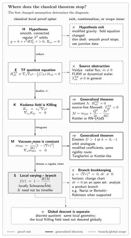
Follow the first changed theory, source, dimension, or orbit assumption in the classical local Birkhoff proof to obtain the primary rigidity diagnosis, then apply the dotted branch and global checks. Dashed multiplication-marked exits show where modified field equations, shells, or genuine spherical sources make that proof unavailable. Double-bordered implication cards show that a constant cosmological term, source-free Maxwell field, and regular higher-dimensional or constant-curvature-orbit analogues instead preserve an appropriately modified theorem. A null areal-radius gradient at a horizon and an open constant-radius product are nested branch questions, while a quotient adds the separate question of whether the local Killing field descends globally. Displayed equations and classifications are exact; the flow layout is schematic.

The same diagnostic is recorded semantically below. Its levels should not be flattened into five mutually exclusive labels. The first three rows give the primary theory-and-source verdict: rigidity can fail, staticity can survive in a different matter family, or an appropriately generalized theorem can survive. The final two rows supply nested qualifications about branch or chart choice and about regularity or global descent. Thus Einstein–$\Lambda$ has a generalized Birkhoff theorem as its primary verdict, while Nariai is a constant-radius branch within that theorem; electrovacuum products are classified in the same two-stage way.

Outcome	What changes?	Representative examples	Correct conclusion
Primary — genuine loss of local symmetry enhancement	Matter or an additional gravitational degree of freedom permits spherical dynamics.	Varying-mass Vaidya; ordinary evolving FLRW; a dynamical canonical scalar; some metric-$f(R)$ branches	The classical theorem is inapplicable, and explicit solutions can lack the additional orbit-space Birkhoff Killing field even when other symmetries remain.
Primary — staticity survives, but the Schwarzschild family does not	Nonvacuum stress obstructs the Kodama proof while another static Killing field remains.	A static perfect-fluid star; a static scalar-supported solution	Nonzero $T_{ab}^{\mathrm{TF}}$ is not a universal no-Killing criterion.
Primary — a generalized Birkhoff theorem survives	Constants, dimension, orbit geometry, field content, or the solution family changes while a rigidity theorem remains.	Einstein–$\Lambda$; source-free electrovac; $D>4$ Einstein gravity; constant-curvature orbit analogues; regular Palatini-$f(R)$ sectors; generic Lovelock branches	State the new hypotheses and classify the new family instead of calling it a failure.
Nested — a branch or chart issue	A coordinate used in a short proof degenerates, or a separate constant-radius branch must be retained.	An ordinary horizon; an isolated bifurcation point; Nariai or Bertotti–Robinson products	After establishing the applicable rigidity theorem, change chart or solve the missing branch; the local enhancement remains.
Nested — a regularity or global limitation	The smooth local theorem applies only piecewise, or a local field fails to descend through a quotient.	A nonnull thin shell; a discrete spacetime quotient	Apply the theorem on each smooth open piece and analyze junction or descent data separately.

The rest of the page works through these rows rather than treating the table as a substitute for analysis.

Genuine spherical dynamics from matter

Vaidya: flux makes the mass a function

In advanced coordinates, the ingoing Vaidya metric is

$$ds^2 =-\left(1-\frac{2Gm(v)}{r}\right)dv^2 +2\,dv\,dr+r^2d\Omega_2^2.$$

Einstein’s equation gives

$$G_{vv}=\frac{2G\dot m(v)}{r^2},$$

and therefore

$$T_{ab} =\frac{\dot m(v)}{4\pi r^2}(dv)_a(dv)_b, \qquad T^{(2)}=0,$$

so the quotient stress is entirely trace free. With the advanced-time convention above, $\dot m\ge0$ satisfies the null energy condition and describes ingoing positive-energy radiation. The Misner–Sharp scalar is exactly $m(v)$, and the mass law reduces to

$$\nabla_a m=\dot m\,(dv)_a.$$

This example also exposes a common curvature shortcut. Null dust has zero trace, so

$$R=0$$

even when $\dot m\ne0$. Vanishing scalar curvature does not imply $R_{\mu\nu}=0$.

When $\dot m=0$, the stress vanishes and $\partial_v$ is Killing. Away from a zero of

$$f(r)=1-\frac{2GM}{r},$$

the substitutions

$$dv=dt+\frac{dr}{f}, \qquad dt=dv-\frac{dr}{f}$$

map the ingoing and diagonal Schwarzschild forms into one another. The factors $1/f$ make this coordinate map invalid at a horizon, but the ingoing metric itself remains regular there. Schleich and Witt show directly that the vacuum equation forces the Vaidya mass function to be constant in 2010, printed p. 4, Eqs. (11)–(12), Open PDF. The historical radiating solution is due to Vaidya 1951; the normalization and signs displayed here follow from the Einstein equation and the retained exact calculation, not from an uninspected equation in that paper.

Vaidya Null-Fluid Spacetimes develops the global and matter interpretation beyond this diagnostic use.

FLRW: zero radial flux is not enough

For an FLRW perfect fluid,

$$ds^2=-dt^2+a(t)^2 \left( \frac{d\chi^2}{1-k\chi^2} +\chi^2d\Omega_2^2 \right), \qquad r=a(t)\chi,$$

and

$$T_{ab}=(\rho+p)u_a u_b+p\,h_{ab}.$$

The quotient trace-free part is

$$T_{ab}^{\mathrm{TF}} =(\rho+p) \left( u_a u_b+\frac12h_{ab} \right).$$

A comoving observer measures no radial energy flux, $T_{t\chi}=0$, yet the Kodama obstruction is nonzero whenever $\rho+p\ne0$. The geometric definition and the first Friedmann equation give the same spherical mass in two useful forms:

$$m_{\mathrm{MS}}=\frac{r^3}{2G}\left(H^2+\frac{k}{a^2}\right)=\frac{4\pi}{3}\rho r^3.$$

Along a comoving sphere, energy conservation gives the exact pressure-work law

$$u(m)=-4\pi p r^2u(r).$$

For dust, $p=0$, each comoving sphere therefore carries constant mass. The spacetime can still expand or contract: that mass is not a constant scalar throughout spacetime, and $T_{ab}^{\mathrm{TF}}\ne0$ when $\rho>0$. At the opposite control value $p=-\rho$, the quotient stress is pure trace. Writing $\Lambda=8\pi G\rho$, its geometrically corrected mass obeys

$$m_{\mathrm{MS}}-\frac{\Lambda r^3}{6G}=0.$$

For $\rho>0$, the resulting de Sitter geometry may be written in time-dependent FLRW coordinates while retaining maximal local symmetry. The controls $\rho=0$ and $\rho<0$ instead give Minkowski space and, in an appropriate open FLRW patch, anti-de Sitter space. Time-dependent metric coefficients are not, by themselves, an invariant diagnosis of dynamical geometry.

The FLRW symmetry and Friedmann evolution are given in Reall 2013, §13.3, printed pp. 158–162, Eqs. (13.28)–(13.42), Open PDF; the pressure-work identity appears in Hayward 1996, printed pp. 12–13, Eqs. (26)–(33), Open PDF. FLRW Spacetimes develops the homogeneous geometry in full.

A scalar: the no-flux trap in its cleanest form

For a canonical scalar with potential $V(\phi)$,

$$T_{\mu\nu} =\nabla_\mu\phi\nabla_\nu\phi -\frac12g_{\mu\nu}(\nabla\phi)^2 -V(\phi)g_{\mu\nu}.$$

On the quotient,

$$T_{ab}^{\mathrm{TF}} =\nabla_a\phi\nabla_b\phi -\frac12h_{ab}(\nabla\phi)^2_h.$$

The potential cancels from the trace-free part. A homogeneous but time-dependent field has $\partial_\chi\phi=0$, hence no comoving radial flux, while its kinetic term still makes $T_{ab}^{\mathrm{TF}}\ne0$.

An exact witness is the flat, massless-scalar FLRW solution for $t>0$,

$$a(t)=a_0\left(\frac{t}{t_0}\right)^{1/3}, \qquad \phi(t) =\phi_0\pm\frac{1}{\sqrt{12\pi G}} \ln\left(\frac{t}{t_0}\right).$$

It satisfies the Einstein–scalar equations, has $p=\rho$, and carries no radial flux. Nevertheless,

$$R=-\frac{2}{3t^2}$$

varies invariantly, so its time dependence cannot be removed by a coordinate change.

More generally, Husain, Martinez, and Núñez exhibit an inhomogeneous spherical Einstein–massless-scalar solution whose nonstatic branch has only the three rotational Killing fields; the nominal time generator is merely conformal Killing 1994, printed pp. 3–4, Eqs. (1)–(6), Open PDF. Scalar-Supported Exact Spacetimes treats the wider solution families.

Staticity can survive nonvacuum matter

Consider a static spherical metric

$$ds^2 =-e^{2\Phi(r)}dt^2 +\frac{dr^2}{A(r)} +r^2d\Omega_2^2.$$

The vector $\partial_t$ is Killing by construction. With a suitable quotient orientation, however, the Kodama field is

$$K=\sqrt{A}\,e^{-\Phi}\,\partial_t.$$

A position-dependent multiple of a Killing field is generally not Killing. Unless $\sqrt A\,e^{-\Phi}$ is constant, the Kodama field therefore fails the Killing test even though the spacetime is manifestly static.

This is exactly why the sourced equation must be interpreted as a proof diagnostic. Static perfect-fluid stars and static scalar configurations can have $T_{ab}^{\mathrm{TF}}\ne0$; matter changes the radial field equations and the local family, but it need not create time dependence. In a timelike polar-areal cell, vanishing radial current together with time-independent density and radial pressure is sufficient for a hypersurface-orthogonal Killing field. Vanishing radial current alone is not sufficient, as Faraoni emphasizes using McVittie as an adverse case 2010, printed pp. 2–3, Eqs. (3)–(15), Open PDF.

The safe conclusion is therefore:

$$T_{ab}^{\mathrm{TF}}\ne0 \quad\Longrightarrow\quad \text{the vacuum Kodama argument is blocked},$$

not

$$T_{ab}^{\mathrm{TF}}\ne0 \quad\Longrightarrow\quad \text{no additional Killing field exists}.$$

Generalized theorems, not failures

Cosmological constant and Maxwell field

A cosmological term is proportional to the metric, so it drops out of the quotient trace-free equation. Birkhoff’s Theorem with a Cosmological Constant consequently obtains the varying-radius Kottler family and the open constant-radius Nariai branch.

Source-free spherical Maxwell stress is also pure trace on the two-dimensional quotient. Electrovac Birkhoff Theorems obtains dyonic Reissner–Nordström–(A)dS together with the supported constant-radius products. The charge and cosmological terms alter the mass correction and solution family, not the local symmetry-enhancement mechanism.

Higher-dimensional Einstein gravity

For round $S^{D-2}$ orbits in $D\ge4$ Einstein gravity, the varying-radius vacuum family has

$$f(r) =1-\frac{\mu}{r^{D-3}} -\frac{2\Lambda r^2}{(D-1)(D-2)}.$$

These limits are worth checking explicitly. At $D=4$ and $\mu=2GM$, this is Kottler. At $D=5$, the mass term falls as $r^{-2}$ and the cosmological coefficient is $-\Lambda r^2/6$. At $\Lambda=0$, it is the Schwarzschild–Tangherlini lapse. For $\Lambda=-(D-1)(D-2)/(2L^2)$, the last term becomes $+r^2/L^2$.

The falloff power and cosmological coefficient change with dimension, but a closely analogous local Killing enhancement remains. In the standard asymptotically flat spherical normalization,

$$\mu =\frac{16\pi G_D M_{\mathrm{ADM}}} {(D-2)\Omega_{D-2}}.$$

Calling $\mu$ an ADM mass outside those asymptotic and normalization assumptions would be unjustified. Schmidt derives the higher-dimensional warped-product symmetry mechanism in 1997, §6, printed pp. 14–16, Eqs. (6.1)–(6.7), Open PDF, while Schwarzschild–Tangherlini Spacetimes develops the detailed normalization and dimensional limits.

Constant-curvature orbit analogues

Replacing round spheres by two-dimensional constant-curvature orbits with $k=0$ or $k=-1$ changes the symmetry hypothesis. In four-dimensional Einstein–$\Lambda$ gravity the local varying-radius form becomes

$$f(r)=k-\frac{2\mu}{r}-\frac{\Lambda r^2}{3}.$$

Here $k$ denotes orbit curvature, not the Kodama vector. For $k=1$ with the usual spherical normalization, $\mu=GM$. For planar or hyperbolic orbits, the physical interpretation of $\mu$ depends on global identifications and normalization; the local equation alone does not turn it into a total mass. These are analogues with different orbit geometry, not counterexamples to the round-$S^2$ theorem. Changing the orbit geometry is distinct from taking a discrete quotient of an unchanged local spacetime.

Changing the field equations

The word “vacuum” is theory-dependent. In metric $f(R)$ gravity, set $f_R=df/dR$ and $T=g^{\mu\nu}T_{\mu\nu}$. The field equation is

$$f_R R_{\mu\nu} -\frac12f g_{\mu\nu} -\nabla_\mu\nabla_\nu f_R +g_{\mu\nu}\Box f_R=8\pi G T_{\mu\nu}.$$

In four dimensions its trace is

$$3\Box f_R+f_R\,R-2f=8\pi G T.$$

On a nonlinear, nondegenerate branch—for example, where $f_{RR}\ne0$—the derivatives in this equation make $f_R$ behave as an additional dynamical scalar. Linear $f(R)=aR+b$ has no such extra scalar degree of freedom. Ordinary $T_{\mu\nu}=0$ therefore does not generally remove every spherical degree of freedom, and some metric-$f(R)$ branches can be genuinely time dependent. This is an existence and mechanism statement, not a claim that every metric-$f(R)$ solution is dynamical.

Palatini $f(R)$ gravity is different. Assume here that the matter action does not depend on the independent connection, and write $\mathcal R$ for the Ricci scalar built from that connection. Its four-dimensional trace equation,

$$f_{\mathcal R}\mathcal R-2f=8\pi G T,$$

is algebraic in $\mathcal R$, rather than a wave equation for $f_{\mathcal R}$. In vacuum or source-free spherical electrovac, a regular isolated root with nonzero $f_{\mathcal R}$ can reduce the equations to Einstein gravity with an effective cosmological constant and, for matter, a rescaled coupling; a generalized Birkhoff theorem then survives. Constant trace alone is not enough: it fixes $\mathcal R$ algebraically but does not make the remaining stress tensor stationary or pure trace on the quotient. Vaidya null dust, for example, has $T=0$ and remains dynamical when $\dot m\ne0$. Faraoni develops the metric-versus-Palatini distinction in 2010, printed pp. 8–9, Eqs. (51)–(53), Open PDF.

Lovelock gravity supplies a sharper warning against vague statements about “higher curvature.” In the source-local coupling convention used by Zegers, generic $C^2$ spherical, planar, or hyperbolic solutions belong to a locally static black-hole family. A genuinely exceptional class appears only at a fine-tuned value $\lambda$ satisfying

$$P(\lambda)=0, \qquad P'(\lambda)=0,$$

where the factorized integrability equation degenerates and an arbitrary two-variable function $B(u,v)$ can remain. Zegers proves both the generic theorem and this exceptional class in 2005, printed pp. 1–4, Eqs. (1)–(37), Open PDF. “Modified gravity violates Birkhoff” is therefore too crude: theory, formulation, coupling branch, and regularity all matter.

Horizons and constant-radius branches

Once the relevant field equations have established that $K$ is Killing—as they do on the vacuum, Einstein–$\Lambda$, and source-free spherical electrovac rigidity branches—the identity

$$K^2=-q, \qquad q=(\nabla r)^2_h,$$

organizes the causal cases without choosing a diagonal chart. Without that dynamical step, it determines only the causal character of the Kodama direction: in a sourced spacetime, $q=0$ can describe a trapping or marginal surface without being a Killing horizon. The following interpretations are therefore restricted to a branch on which the extra Killing symmetry has already been proved.

Invariant situation	What happens?	Interpretation
$q>0$	$K$ is timelike.	A local static cell exists.
$q=0$ and $dr\ne0$	$K$ is nonzero and null.	This is an ordinary Killing-horizon point; use a horizon-regular chart.
$q<0$	$K$ is spacelike.	The local solution can be homogeneous rather than static, while $K$ remains Killing.
$dr=0$ at an isolated point	$K=0$ there.	In the relevant analytic Schwarzschild-family extension, this is a bifurcation-type critical point, not an open product.
$dr=0$ on an open set	The Kodama field vanishes throughout that set.	Solve the constant-radius field equations separately; another factor symmetry supplies the enhancement when the branch exists.

The diagonal transformation $dt=dv-dr/f$ divides by $f$ and therefore cannot prove anything at $f=0$. Conversely, the regular advanced metric has determinant $-1$ in its $(v,r)$ block and passes smoothly through an ordinary root. Losing the static chart at a horizon is not losing the Killing field.

An open constant-radius region is genuinely a separate solution branch. Vacuum Einstein gravity with round $S^2$ orbits admits no such finite-radius branch, but Einstein–$\Lambda$ admits Nariai and electrovac admits Bertotti–Robinson and charged Nariai-type products. Directly substituting a degenerate horizon radius into a diagonal black-hole metric does not produce the product geometry; a near-horizon scaling is required. The preceding $\Lambda$ and electrovac pages give the exact branch equations and limiting procedures.

Shells and global identifications

A thin shell is piecewise vacuum

A nonnull spherical thin shell has a continuous induced metric but a finite jump in transverse first derivatives, equivalently in extrinsic curvature. In Gaussian normal coordinates adapted across the shell, the first junction condition can be written

$$[g_{\mu\nu}]=0,$$

which asserts continuity of the metric, not of its transverse derivative. Its surface stress tensor is a delta-function source. Choose one unit normal $n^\mu$ directed from the minus side to the plus side, set $\epsilon=n^\mu n_\mu$ and $[Q]=Q_+-Q_-$, and define $K_{ij}=-e_i^\mu e_j^\nu\nabla_\mu n_\nu$, where $e_i^\mu$ are tangent vectors to the shell and $h_{ij}$ is its induced metric. With $K=h^{ij}K_{ij}$, the junction law is

$$8\pi G\,S_{ij} =\epsilon\left([K_{ij}]-h_{ij}[K]\right).$$

The smooth vacuum theorem applies separately on the two open sides. Each side can be locally Schwarzschild, while the mass parameters may differ; the junction data determine their relation. No single smooth-vacuum argument is allowed to cross the layer and force the two constants to agree.

Israel derives the nonnull surface-layer law and the spherical shell specialization in 1966, printed pp. 7–14, Eqs. (19)–(43); his extrinsic-curvature sign is opposite to the one displayed here. Bičák explicitly describes a spherical shell separating Schwarzschild regions of masses $M$ and $M+m$ in 2000, §2.3, printed pp. 23–24, Open PDF. Darmois–Israel Junction Conditions gives the full sign-translated derivation. Null layers require different transverse-curvature data; see Null Junction Conditions.

Lower regularity alone is not a counterexample. It means that a particular classical proof no longer applies. Establishing a failure at low regularity would require a precisely formulated weak theorem and an example violating its conclusion.

Local Killing fields need not descend globally

Let $\widetilde M$ be a covering spacetime and $M=\widetilde M/\Gamma$ a discrete quotient. A vector field $\widetilde K$ descends to $M$ exactly when it is invariant under every deck transformation:

$$\gamma_*\widetilde K=\widetilde K \qquad \text{for every }\gamma\in\Gamma.$$

Equivalently, a one-parameter isometry flow must normalize the deck group to induce a quotient isometry. If this condition fails, every sufficiently small neighborhood can still be locally Schwarzschild or Kottler even though the corresponding Killing flow is not globally defined on the quotient.

Schleich and Witt analyze Schwarzschild, de Sitter, and other quotient examples and list the global properties that a local Birkhoff theorem does not determine in 2009, Examples 1–8, conclusion, and Appendix Theorem 2, printed pp. 3–18, Open PDF. Coordinate Form versus Local Isometry develops the local-isometry distinction.

A practical decision procedure

When a spherical metric is advertised as a Birkhoff counterexample, ask these questions in order.

1. Which field equations? Separate Einstein, Einstein–$\Lambda$, Einstein–Maxwell, scalar–tensor, metric or Palatini $f(R)$, Lovelock, and other theories.
2. Which source sector? Compute the full quotient stress, not merely one radial-flux component or the four-dimensional trace.
3. Which dimension and orbit geometry? Round $S^2$, $S^{D-2}$, planar, and hyperbolic orbits lead to different local families and mass normalizations.
4. Which regularity domain? Identify smooth open regions, nonnull shells, null layers, and any weak formulation before differentiating the metric.
5. Which areal-radius branch? Distinguish $q=0$ with $dr\ne0$, isolated $dr=0$, and $dr=0$ on an open set.
6. Which conclusion is claimed? An extra local Killing field is weaker than a global static region, asymptotic flatness, a preferred maximal extension, or a globally defined time translation.

Only an example satisfying the same hypotheses and lacking the theorem’s local conclusion would refute the theorem. Most familiar “exceptions” instead reveal why one of its assumptions is indispensable.

Common pitfalls

“No radial flux” means vacuum. A comoving FLRW fluid and a homogeneous scalar have zero radial flux but nonzero quotient trace-free stress. Inspect $T_{ab}^{\mathrm{TF}}$, the mass law, and the remaining field equations.

A non-Killing Kodama field means the spacetime is time dependent. It means only that the vacuum Kodama proof is unavailable. A static star can possess a different Killing field.

Time-dependent coefficients prove physical evolution. De Sitter space has time-dependent FLRW slicings. Use curvature invariants, matter scalars, and Killing equations rather than coordinate appearance.

A horizon violates staticity and hence Birkhoff. At a regular horizon the additional field is null, not absent. The diagonal chart fails because it divided by the lapse.

Every higher-curvature theory behaves alike. Metric and Palatini $f(R)$ differ, and generic Lovelock branches retain a theorem while a precise fine-tuned branch can evade it.

Vacuum on both sides means one mass across a shell. The shell is distributional matter. Birkhoff fixes one constant on each connected smooth vacuum side; junction conditions relate, but need not equal, those constants.

Exercises

1. Diagnose ingoing Vaidya

For

$$ds^2 =-\left(1-\frac{2Gm(v)}r\right)dv^2 +2\,dv\,dr+r^2d\Omega_2^2,$$

show that $m_{\mathrm{MS}}=m(v)$, explain why $R=0$ does not imply vacuum, and recover Schwarzschild when $\dot m=0$.

Solution

The inverse quotient metric has $h^{rr}=1-2Gm/r$, so

$$q=(\nabla r)^2=1-\frac{2Gm(v)}r.$$

Therefore

$$m_{\mathrm{MS}} =\frac{r}{2G}(1-q)=m(v).$$

Einstein’s equation gives null stress

$$T_{ab} =\frac{\dot m}{4\pi r^2}(dv)_a(dv)_b.$$

Because $dv$ is null with respect to the inverse quotient metric, $T^\mu{}_\mu=0$, hence $R=-8\pi G T^\mu{}_\mu=0$. The Ricci tensor is nevertheless nonzero when $\dot m\ne0$. If $\dot m=0$, the stress vanishes and $\partial_v$ is Killing. Where $f\ne0$, substituting $dt=dv-dr/f$ gives the diagonal Schwarzschild form; the ingoing form itself remains regular at an ordinary horizon.

2. Separate FLRW mass conservation from Birkhoff rigidity

For a comoving FLRW perfect fluid, derive $T_{ab}^{\mathrm{TF}}$ and the pressure-work law. Explain the dust and $p=-\rho$ controls.

Solution

On the quotient,

$$T_{ab}=(\rho+p)u_a u_b+p h_{ab}, \qquad T^{(2)}=-\rho+p.$$

Subtracting half the trace gives

$$T_{ab}^{\mathrm{TF}} =(\rho+p) \left(u_a u_b+\frac12h_{ab}\right).$$

The Friedmann equation yields $m=4\pi\rho r^3/3$. Along a comoving sphere, $u(r)=Hr$ and $u(\rho)=-3H(\rho+p)$, so

$$\begin{aligned} u(m) &=\frac{4\pi}{3} \left[r^3u(\rho)+3\rho r^2u(r)\right] \\ &=-4\pi p r^2u(r). \end{aligned}$$

For dust, $p=0$, a chosen comoving sphere has constant mass, but $T_{ab}^{\mathrm{TF}}\ne0$ and the geometry can evolve. For $p=-\rho$, the trace-free block vanishes and stress conservation makes $\rho$ constant. This is vacuum energy: the FLRW geometry is locally de Sitter for $\rho\gt0$, Minkowski for $\rho=0$, and anti-de Sitter for $\rho\lt0$, even when the chosen slicing is time dependent. The cosmological volume term must be subtracted before expecting a conserved Birkhoff mass.

3. Build a zero-flux scalar counterexample

Verify that

$$a(t)=a_0(t/t_0)^{1/3}, \qquad \phi(t)=\phi_0+\frac{1}{\sqrt{12\pi G}}\ln(t/t_0)$$

solves the flat FLRW Einstein equations for a massless canonical scalar. Why does it defeat the statement “zero radial flux restores Birkhoff”?

Solution

The scalar derivative is

$$\dot\phi=\frac{1}{\sqrt{12\pi G}\,t},$$

so

$$\rho=p=\frac12\dot\phi^2 =\frac{1}{24\pi Gt^2}.$$

For $a\propto t^{1/3}$, $H=1/(3t)$, and

$$H^2=\frac{1}{9t^2} =\frac{8\pi G}{3}\rho.$$

The scalar equation $\ddot\phi+3H\dot\phi=0$ also holds. Homogeneity gives $T_{t\chi}=\dot\phi\,\partial_\chi\phi=0$, but

$$T_{ab}^{\mathrm{TF}} =\nabla_a\phi\nabla_b\phi -\frac12h_{ab}(\nabla\phi)^2_h$$

is nonzero. Moreover $R=-2/(3t^2)$ varies, proving genuine invariant evolution. Zero radial flux removed one tensor component, not the scalar kinetic degree of freedom.

4. Classify the alleged exceptions

Give the primary theory-and-source verdict for each case, then add a nested branch, regularity, or global qualification where needed: (a) Einstein–$\Lambda$, (b) source-free spherical Maxwell, (c) a static perfect-fluid star, (d) a simple Schwarzschild horizon, (e) a Nariai open product, (f) a timelike spherical shell, (g) a nontrivial quotient of a locally Schwarzschild region, (h) generic Lovelock couplings, (i) $P(\lambda)=P'(\lambda)=0$ in the Lovelock convention above, and (j) a dynamical metric-$f(R)$ branch.

Solution

• Generalized theorem: (a) gives the Kottler and Nariai branches; (b) gives Reissner–Nordström–(A)dS and the charged product branches; (h) retains the generic Lovelock theorem. Case (e) therefore has this same primary Einstein–$\Lambda$ verdict.
• Changed static family: (c) is nonvacuum and not Schwarzschild, but it retains a static Killing field.
• Genuine local symmetry loss is permitted: (i) is the fine-tuned Lovelock degeneracy with arbitrary two-variable data; (j) can retain a dynamical scalar gravitational mode. An explicit solution is still needed to prove that a particular metric in either theory actually lacks the additional orbit-space Birkhoff Killing field.
• Nested branch or chart qualifications: (d) lies in the ordinary vacuum Schwarzschild family but its Killing field is null at the horizon, so a regular chart is required; (e) is the open constant-radius branch nested inside the Einstein–$\Lambda$ theorem rather than a separate primary failure.
• Nested regularity or global qualifications: (f) is piecewise smooth with distributional surface stress, so the vacuum-family conclusion applies separately on the two sides; (g) preserves the local Schwarzschild family but may obstruct global descent of its Killing flow.

References

• Bičák, Jiří. “Selected Solutions of Einstein’s Field Equations: Their Role in General Relativity and Astrophysics.” In Einstein’s Field Equations and Their Physical Implications, Lecture Notes in Physics 540, 1–126. Berlin: Springer, 2000. doi:10.1007/3-540-46580-4_1. Open PDF.
• Faraoni, Valerio. “The Jebsen–Birkhoff Theorem in Alternative Gravity.” Physical Review D 81 (2010), 044002. doi:10.1103/PhysRevD.81.044002. Open PDF.
• Hayward, Sean A. “Gravitational Energy in Spherical Symmetry.” Physical Review D 53 (1996), 1938–1949. doi:10.1103/PhysRevD.53.1938. Open PDF.
• Husain, Viqar, Erik A. Martinez, and Darío Núñez. “Exact Solution for Scalar Field Collapse.” Physical Review D 50 (1994), 3783–3786. doi:10.1103/PhysRevD.50.3783. Open PDF.
• Israel, Werner. “Singular Hypersurfaces and Thin Shells in General Relativity.” Il Nuovo Cimento B 44 (1966), 1–14; erratum 48 (1967), 463. Article doi:10.1007/BF02710419. Erratum doi:10.1007/BF02712210.
• Reall, Harvey S. General Relativity. Cambridge Part III lecture notes, 2013. Official PDF.
• Schleich, Kristin, and Donald M. Witt. “A Simple Proof of Birkhoff’s Theorem for Cosmological Constant.” Journal of Mathematical Physics 51 (2010), 112502. doi:10.1063/1.3503447. Open PDF.
• Schleich, Kristin, and Donald M. Witt. “What Does Birkhoff’s Theorem Really Tell Us?” arXiv:0910.5194v1 [gr-qc] (2009). arXiv record. Open PDF.
• Schmidt, Hans-Jürgen. “A New Proof of Birkhoff’s Theorem.” Gravitation and Cosmology 3 (1997), 185–190. Open PDF.
• Vaidya, Prahalad Chunnilal. “The Gravitational Field of a Radiating Star.” Proceedings of the Indian Academy of Sciences, Section A 33 (1951), 264–276. doi:10.1007/BF03173260.
• Zegers, Robin. “Birkhoff’s Theorem in Lovelock Gravity.” Journal of Mathematical Physics 46 (2005), 072502. doi:10.1063/1.1960798. Open PDF.