The Vacuum Birkhoff Theorem

Spherical symmetry alone does not freeze a spacetime: FLRW cosmologies and Vaidya radiation are spherical and time dependent. Vacuum is the decisive extra hypothesis. It forces the Hessian of the areal radius to be pure trace, turns the Kodama direction into a genuine Killing field, and makes the spherical mass constant. The result is local Schwarzschild geometry—but the new Killing field is timelike only in a static region, null on an ordinary horizon branch, zero at a bifurcation sphere, and spacelike in a black-hole interior.

Required background. The Einstein Equation supplies the vacuum reduction; Killing Fields and Isometry Groups supplies the Killing and hypersurface-orthogonality criteria.

Helpful background. The Riemann Curvature Tensor supports the warped-product identities; Formulations of General Relativity supplies alternative coordinate and initial-value proofs.

Within this chapter. Spherical Orbit-Space Geometry introduces the quotient $(Q,h)$, the invariant areal radius $r$, its volume form $\epsilon_{ab}$, and the Kodama vector. Areal Radius and Spherical Mass Functions derives the Misner–Sharp definition and its matter-flux law. The proof below specializes those two constructions to vacuum.

The precise local theorem

Let $\mathcal U$ be a connected $C^3$, four-dimensional, time-oriented Lorentzian region satisfying

$$R_{\mu\nu}=0.$$

Assume that $\mathcal U$ carries an effective local $SO(3)$ isometric action whose orbits are spacelike round two-spheres. Thus $\mathcal U$ is a regular-orbit region with $r>0$; it may contain a horizon or a critical point of $r$, but it does not include a symmetry center as an ordinary two-sphere orbit. The $C^3$ threshold is a sufficient working hypothesis for the classical curvature and differentiated identities below, not a claim of optimal low-regularity sharpness.

Then there is one constant $M$ such that every point of $\mathcal U$ has a neighborhood locally isometric to the Schwarzschild solution with mass parameter $M$. The same $M$ applies throughout the connected region. In addition to the three rotational generators, the metric has a hypersurface-orthogonal local Killing field $K$ orthogonal to the symmetry spheres.

The conclusion includes $M>0$, $M=0$, and $M<0$. It assumes neither asymptotic flatness nor a regular center, event horizon, maximal extension, preferred topology, formation history, or stability. Those extra conditions can restrict the mass or the global spacetime, but they are not consequences of this local field-equation theorem. A branch-complete null-coordinate proof is given in Schleich and Witt 2010, Theorem 1 and proof, arXiv v2 pp. 3–4, Eqs. (4)–(12), Open PDF. Hayward independently integrates the vacuum double-null equations directly to Kruskal form in Hayward 1996, printed p. 7, Proposition 4 and Eqs. (12)–(14), Open PDF.

The reduced equations that carry the proof

On the regular spherical quotient, write

$$g=h_{ab}(x)dx^a dx^b+r^2(x)d\Omega_2^2, \qquad q=(\nabla r)^2_h.$$

Indices $a,b$ refer to the two-dimensional quotient and $i,j$ to the unit two-sphere. Here $\nabla$ is the Levi–Civita connection of $h$, and $\Box_h=h^{ab}\nabla_a\nabla_b$.

The warped-product Ricci tensor has the blocks

$$R^{(4)}_{ab} =R^{(h)}_{ab}-\frac{2}{r}\nabla_a\nabla_b r,$$ $$R^{(4)}_{ij} =\left(1-q-r\Box_h r\right)\gamma_{ij},$$

where $\gamma_{ij}$ is the unit-sphere metric. In two dimensions, $R^{(h)}_{ab}=\tfrac12 R_h h_{ab}$. Therefore the trace-free part of $R^{(4)}_{ab}=0$ and the angular vacuum equation are respectively

$$\nabla_a\nabla_b r =\frac12(\Box_h r)h_{ab}, \tag{1}$$ $$1-q-r\Box_h r=0. \tag{2}$$

The trace of the quotient block also gives

$$R_h=\frac{2}{r}\Box_h r.$$

Equations (1) and (2) are the load-bearing relations for the extra symmetry and constant mass; this trace relation completes the curvature reconstruction. No static coordinate ansatz has been used.

Before imposing vacuum, the kinematic construction is worth seeing. In the figure, inspect the lower cards: $K={}^\star dr$ is orthogonal to $dr$ and has the opposite squared norm. The diagram does not assert that $K$ is Killing; that is the new content of Eq. (1).

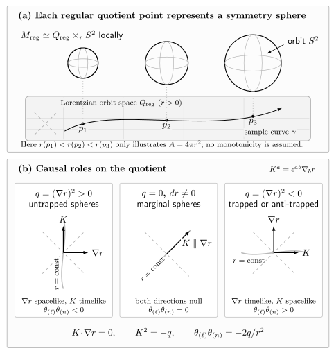
The quotient and causal cards show the kinematic identities $K^a=\epsilon^{ab}\nabla_b r$, $K^a\nabla_a r=0$, and $K^2=-(\nabla r)^2$. These hold in any sufficiently regular spherically symmetric spacetime. Vacuum supplies the separate pure-trace Hessian equation that makes $K$ Killing; the schematic figure does not itself prove that dynamical step. The center $r=0$ and global topology lie outside the regular-fiber picture.

Vacuum turns Kodama into a Killing field

Lower the Kodama vector on $Q$:

$$K_a=\epsilon_a{}^b\nabla_b r.$$

The quotient volume form is covariantly constant. If $H_{ab}=\nabla_a\nabla_b r$, then

$$\nabla_aK_b=\epsilon_b{}^cH_{ac}.$$

Using Eq. (1) gives the complete Killing calculation:

$$\begin{aligned} \nabla_{(a}K_{b)} &=\frac12\left( \epsilon_b{}^cH_{ac}+\epsilon_a{}^cH_{bc} \right)\\ &=\frac14(\Box_h r) \left(\epsilon_{ba}+\epsilon_{ab}\right)\\ &=0. \end{aligned}$$

Thus $K$ is Killing even though no time independence was assumed. It is also hypersurface-orthogonal: $K^\flat$ has components only on the two-dimensional quotient, so $K^\flat\wedge dK^\flat=0$ there and after the spherical lift. The extra symmetry is therefore locally static wherever $K$ is timelike—but not where it is null, zero, or spacelike.

The displayed calculation proves the quotient components of the Killing equation. The lift is just as important: antisymmetry gives $K(r)=0$, so

$$(\mathcal L_K g)_{ij}=2rK(r)\gamma_{ij}=0,$$

and the mixed quotient–sphere components vanish because the warped product has no mixed block. Hence $\mathcal L_Kg=0$ for the full four-dimensional metric, not merely for $h$.

This is the logical step that fails for generic spherical matter. The Kodama vector still exists, but the trace-free quotient stress can make $H_{ab}$ anisotropic and hence $\nabla_{(a}K_{b)}\ne0$.

Vacuum makes the mass constant

Define the spherical mass by

$$m=\frac{r}{2G}(1-q).$$

This is the Misner–Sharp mass: Hayward gives the same invariant definition in $G=1$ units in Hayward 1996, printed p. 4, Eq. (4), Open PDF.

Equation (1) first gives

$$\nabla_a q =2(\nabla_a\nabla_b r)\nabla^b r =(\Box_h r)\nabla_a r.$$

Differentiating $m$ and then using Eq. (2),

$$\begin{aligned} \nabla_a m &=\frac{1}{2G} \left[(1-q)-r\Box_h r\right]\nabla_a r\\ &=0. \end{aligned}$$

Connectedness now matters: $m=M$ is one constant on $\mathcal U$, not a chart-by-chart label. Consequently,

$$q=(\nabla r)^2 =1-\frac{2GM}{r} \equiv f(r). \tag{3}$$

The double-null mass-variation equation gives the same conclusion directly: its right-hand side is matter flux and therefore vanishes in vacuum Hayward 1996, printed pp. 6–7, Eqs. (9)–(11), Open PDF.

The zero-mass member is locally Minkowski. A negative-mass member is also locally Ricci-flat; ruling it out requires additional global hypotheses such as a suitable complete asymptotically flat end and a positive-mass theorem. The local equations alone do not choose $M\ge0$.

Coordinates without losing the horizon

Where $dr\ne0$ and $f\ne0$, the vectors $K$ and $\nabla r$ form an orthogonal quotient frame. Hypersurface orthogonality lets us choose $t$ so that $K=\partial_t$ and the $t=\text{constant}$ curves are orthogonal to its flow; equivalently, a residual shift $t\mapsto t+\psi(r)$ removes the cross term. Then $K^2=-f$ and $(\nabla r)^2=f$ fix the quotient metric as $-f\,dt^2+dr^2/f$. On this overlap, defining advanced and retarded coordinates by

$$dv=dt+\frac{dr}{f}, \qquad du=dt-\frac{dr}{f},$$

gives two metric forms whose coefficients remain regular at $f=0$:

$$ds^2=-f(r)dv^2+2\,dv\,dr+r^2d\Omega_2^2. \tag{4a}$$ $$ds^2=-f(r)du^2-2\,du\,dr+r^2d\Omega_2^2. \tag{4b}$$

This regularity of the formulas is not, by itself, a proof that an arbitrary vacuum metric already containing a horizon point is their continuation. The missing existence step is supplied by integrating the reduced vacuum equations directly in $(v,r)$ or $(u,r)$ coordinates wherever $dr\ne0$; this does not divide by $f$. Schleich and Witt carry out that null-coordinate integration in Schleich and Witt 2010, Theorem 1 and proof, arXiv v2 pp. 3–4, Eqs. (4)–(12), Open PDF. It yields Eq. (4a) on one orientation and Eq. (4b) on the other, with the same constant $M$ fixed above.

The advanced coordinate $v$ therefore crosses one horizon branch and the retarded coordinate $u$ crosses the complementary branch. Each radial block has determinant $-1$, including at $f=0$. Neither one-sided chart contains the bifurcation sphere. Conversely, only where $f\ne0$ may one recover

$$dt=dv-\frac{dr}{f} =du+\frac{dr}{f}$$

to obtain the familiar diagonal chart

$$ds^2=-f(r)dt^2+\frac{dr^2}{f(r)}+r^2d\Omega_2^2. \tag{5}$$

The distinction between $dr$ and its norm is essential:

Invariant situation	Local description	What fails
$dr\ne0$ and $f\ne0$	The null forms (4a)–(4b) and diagonal form (5) work. $K$ is timelike for $f>0$ and spacelike for $f<0$.	Nothing; the diagonal chart is merely regime-dependent.
$dr\ne0$ and $f=0$	One of Eqs. (4a)–(4b) is regular on each horizon branch; $K$ is a nonzero null vector.	The diagonal transformation divides by $f$.
$dr=0$ at an isolated point of $Q$	For $M>0$, its four-dimensional preimage is the bifurcation two-sphere at $r=2GM$; a two-null or Kruskal-type chart is needed and $K=0$.	Neither $r$ nor one-sided Eddington–Finkelstein time is a coordinate system at the bifurcation sphere.
$dr=0$ on an open set	No finite-radius vacuum branch exists when $\Lambda=0$.	Assuming $r$ is a coordinate would hide the branch test rather than perform it.

At an isolated vacuum critical point of $r$ on $Q$, Eqs. (1)–(3) imply $M>0$, $r=2GM$, and

$$\nabla_a\nabla_b r =\frac{1}{4GM}h_{ab}.$$

The quotient Hessian is nondegenerate, so the critical point is a Lorentzian saddle. Its four-dimensional preimage is the Schwarzschild bifurcation sphere. To close this branch without dividing by $dr$, set $\mu=GM>0$ and choose normalized double-null coordinates $(U,V)$ in which

$$UV=\left(1-\frac{r}{2\mu}\right)e^{r/(2\mu)}, \qquad h=-\frac{32\mu^3}{r}e^{-r/(2\mu)}\,dU\,dV. \tag{6}$$

At the quotient point $U=V=0$, the implicit relation gives $r=2\mu$, while the metric coefficient tends to the finite nonzero value $-16\mu^2/e$. Differentiating the first relation gives

$$V\,dU+U\,dV =-\frac{r}{4\mu^2}e^{r/(2\mu)}dr,$$

so $dr=0$ at the origin. Up to the choice of quotient orientation, the extra Killing field is

$$K=\frac{1}{4\mu} \left(V\partial_V-U\partial_U\right). \tag{7}$$

It is nonzero and null when exactly one of $U,V$ vanishes, but it vanishes when both do. Thus the two ordinary horizon branches and the quotient point beneath their bifurcation sphere are all present in one regular local chart. Equation (6) is Hayward’s integrated vacuum solution; the statements $dr=0$ and $K=0$ at the origin follow from his equations rather than being asserted separately in the source Hayward 1996, printed p. 7, Proposition 4 and Eqs. (12)–(14); Appendix B, printed pp. 19–20, Eqs. (B1)–(B8), Open PDF.

The Schwarzschild Coordinate Atlas shows which standard charts contain one horizon branch and which contain the bifurcation sphere. Bičák gives the areal and ingoing forms in Bičák 2000, §§2.1–2.3, printed pp. 19–23, especially Eqs. (1), (2), and (4), Open PDF, then the Kruskal form and bifurcation structure in Bičák 2000, §2.4, printed pp. 24–27, Eqs. (5)–(7), Open PDF.

Finally, suppose $dr=0$ on an open set with finite $r>0$. Then $q=0$, $\Box_h r=0$, and the angular Ricci block becomes

$$R^{(4)}_{ij}=\gamma_{ij}\ne0.$$

So vacuum with $\Lambda=0$ has no open constant-radius branch. With positive cosmological constant the equation changes and the Nariai branch becomes possible; that is treated on Birkhoff’s Theorem with a Cosmological Constant.

What the theorem does—and does not—say

The invariant conclusion is additional local symmetry plus local Schwarzschild geometry. It is not “static everywhere.” The causal character follows immediately from

$$K^2=-f(r),$$

For $M>0$, $K$ is timelike for $r>2GM$, a nonzero null generator on an ordinary horizon branch, zero at the bifurcation sphere, and spacelike for $0<r<2GM$. For $M=0$ or $M<0$, $f>0$ at every $r>0$, so there is no positive-radius horizon or interior branch. Faraoni discusses why the coordinate-static statement must be restricted to regions where the additional Killing field is timelike in Faraoni 2010, arXiv v1 pp. 2–3, Eqs. (3)–(15), Open PDF.

Nor does local Schwarzschild form select the maximal Schwarzschild extension. Restricted domains and discrete quotients can have the same local metric but different topology, asymptotics, or extendibility. An exactly spherical vacuum region has no spherical radiative degree of freedom, but the theorem says nothing about nonspherical perturbations, formation, or nonlinear stability.

Matter changes the decisive equation. A Vaidya mass $M(v)$ has radial null flux and is not vacuum when $dM/dv\ne0$; an FLRW fluid is spherical about every comoving observer but need not be stationary. A systematic comparison appears on When Birkhoff’s Conclusion Fails.

Common pitfalls

“Birkhoff means static everywhere.” It guarantees a hypersurface-orthogonal Killing field. Staticity requires that field to be timelike, which fails in the Schwarzschild interior and on the horizon.

“The proof excludes the horizon.” Only the diagonal Schwarzschild chart excludes $f=0$. The two null forms (4a)–(4b) cover the ordinary horizon branches where $dr\ne0$; the Kruskal form (6) also handles the bifurcation point where $dr=0$.

“A null radius gradient is a critical point.” Null means $(\nabla r)^2=0$; critical means the covector $dr$ itself vanishes. A generic horizon point has the first property but not the second.

“The mass must be positive.” Positivity is a global theorem with extra hypotheses. Vacuum Birkhoff admits every real integration constant locally.

Exercises

1. Vacuum upgrades the Kodama field

Starting from $K_a=\epsilon_a{}^b\nabla_b r$ and Eq. (1), show directly that $K$ is Killing.

Solution

Because $\nabla_a\epsilon_{bc}=0$,

$$\nabla_aK_b =\epsilon_b{}^c\nabla_a\nabla_c r =\frac12(\Box_h r)\epsilon_{ba}.$$

Symmetrization removes the antisymmetric volume form:

$$\nabla_{(a}K_{b)} =\frac14(\Box_h r)(\epsilon_{ba}+\epsilon_{ab})=0.$$

For the spherical lift, $K(r)=0$ and therefore $(\mathcal L_Kg)_{ij}=2rK(r)\gamma_{ij}=0$; the mixed components vanish as well. Thus the lifted four-dimensional vector is Killing.

The quotient calculation would not vanish for a generic trace-free part of the Hessian, which is why spherical symmetry without vacuum is insufficient.

2. A horizon is not a critical point

Assume $M>0$. For the radial block of Eq. (4a), compute the inverse metric, $(\nabla r)^2$, and $K^2$ at $r=2GM$. Then use Eqs. (6)–(7) to contrast this ordinary horizon point with $U=V=0$.

Solution

The radial metric and its inverse are

$$h_{ab}= \begin{pmatrix} -f&1\\ 1&0 \end{pmatrix}, \qquad h^{ab}= \begin{pmatrix} 0&1\\ 1&f \end{pmatrix}.$$

Since $dr=(0,1)$ in $(v,r)$ coordinates,

$$(\nabla r)^2=h^{rr}=f.$$

Choose the quotient orientation so that $K=\partial_v$. Then $K^2=h_{vv}=-f$. At $r=2GM$, both norms vanish, but $dr=(0,1)$ and $K=(1,0)$ remain nonzero. This chart covers a regular horizon branch.

By contrast, differentiating Eq. (6) at $U=V=0$ gives $dr=0$, because the derivative of its right-hand side with respect to $r$ is $-e/(2GM)\ne0$. Equation (7) gives $K=0$ there as well. This is the quotient point whose sphere fiber is the bifurcation sphere, not an ordinary point on either one-sided horizon chart.

3. Exclude an open constant-radius vacuum branch

Set $dr=0$ on an open region with $r=r_0>0$. Use the reduced Ricci equations to show that vacuum is impossible when $\Lambda=0$.

Solution

On an open constant-radius region,

$$q=0, \qquad \nabla_a\nabla_b r=0, \qquad \Box_h r=0.$$

The angular block is therefore

$$R^{(4)}_{ij} =(1-q-r\Box_h r)\gamma_{ij} =\gamma_{ij},$$

which cannot vanish for a finite round sphere. Equivalently, the quotient Einstein block contains $-h_{ab}/r_0^2$. Positive $\Lambda$ can balance this curvature and produces the separate Nariai branch; ordinary vacuum cannot.

4. Locate the failed Vaidya hypothesis

Replace $M$ in Eq. (4a) by $\mathcal M(v)$. Show why the result is not a vacuum counterexample to Birkhoff’s theorem.

Solution

For

$$f(v,r)=1-\frac{2G\mathcal M(v)}{r},$$

direct curvature calculation gives

$$R_{vv}=\frac{2G}{r^2}\frac{d\mathcal M}{dv}, \qquad R=0.$$

Einstein’s equation therefore yields the ingoing null-fluid component

$$T_{vv}=\frac{1}{4\pi r^2}\frac{d\mathcal M}{dv}.$$

Also $\partial_vg_{vv}=2G\mathcal M'(v)/r$, so $\partial_v$ is not Killing unless $\mathcal M$ is constant. When $d\mathcal M/dv=0$, the stress vanishes and Eq. (4a) returns to Schwarzschild exactly.

Extensions and next steps

• Birkhoff’s Theorem with a Cosmological Constant adds Kottler and the exceptional Nariai product branch.
• Electrovac Birkhoff Theorems keeps spherical symmetry but adds the Maxwell charge and its stress tensor.
• When Birkhoff’s Conclusion Fails organizes matter, modified-gravity, regularity, dimension, and topology changes by the hypothesis they remove.
• The Maximal Schwarzschild Extension studies the global spacetime that the local theorem deliberately does not select.

References

• Bičák, Jiří. “Selected Solutions of Einstein’s Field Equations: Their Role in General Relativity and Astrophysics.” In Einstein’s Field Equations and Their Physical Implications, Lecture Notes in Physics 540 (Springer, 2000), 1–126. doi:10.1007/3-540-46580-4_1. Open PDF, arXiv:gr-qc/0004016v1.
• Faraoni, Valerio. “The Jebsen–Birkhoff Theorem in Alternative Gravity.” Physical Review D 81 (2010), 044002. doi:10.1103/PhysRevD.81.044002. Open PDF, arXiv:1001.2287v1.
• Hayward, Sean A. “Gravitational Energy in Spherical Symmetry.” Physical Review D 53 (1996), 1938–1949. doi:10.1103/PhysRevD.53.1938. Open PDF, arXiv:gr-qc/9408002v2.
• Schleich, Kristin, and Donald M. Witt. “A Simple Proof of Birkhoff’s Theorem for Cosmological Constant.” Journal of Mathematical Physics 51 (2010), 112502. doi:10.1063/1.3503447. Open PDF, arXiv:0908.4110v2.