Electrovac Birkhoff Theorems

Source-free electric or magnetic flux does not destroy Birkhoff’s symmetry enhancement. In spherical Einstein–Maxwell theory, the quotient part of the Maxwell stress tensor is pure trace, so the same geometric construction that works in vacuum produces an additional local Killing field. The complete answer has two branches: a varying-radius Reissner–Nordström–(anti-)de Sitter branch and a constant-radius family containing Bertotti–Robinson, charged Nariai, and an ultracold flat-factor limit. The theorem is local; it does not turn every root of the metric function into a globally defined black-hole horizon.

Required background. The Einstein Equation supplies Einstein–Maxwell coupling; Killing Fields and Isometry Groups supplies the local-staticity conclusion.

Helpful background. The Riemann Curvature Tensor supports the reduced curvature check; Formulations of General Relativity supplies complementary constraint and flux descriptions.

Within this chapter. Spherical Orbit-Space Geometry defines the quotient metric, areal radius, and Kodama direction; Areal Radius and Spherical Mass Functions develops the invariant mass used below; Birkhoff’s Theorem with a Cosmological Constant treats the uncharged limit and its Nariai branch.

The local electrovac theorem

Let $U$ be a connected, smooth, oriented and time-oriented four-dimensional Lorentzian region satisfying

$$G_{\mu\nu}+\Lambda g_{\mu\nu}=8\pi G T^{\mathrm{EM}}_{\mu\nu},$$ $$T^{\mathrm{EM}}_{\mu\nu} =\frac1{4\pi} \left(F_{\mu\alpha}F_\nu{}^\alpha -\frac14g_{\mu\nu}F_{\alpha\beta}F^{\alpha\beta}\right), \qquad dF=0,\quad d{*F}=0.$$

Assume that an effective local $SO(3)$ action has spacelike round two-sphere orbits of positive area $4\pi r^2$. There are no currents and no other matter fields on $U$. No separate Maxwell symmetry assumption is needed. For a source-free Einstein–Maxwell field, an isometry can change $F$ only by a duality rotation; this defines a homomorphism from the isometry group to a one-parameter group. The Lie algebra of $SO(3)$ is Bianchi type IX and equals its own derived algebra, so that homomorphism is trivial and $\mathcal L_XF=0$ for every spherical generator $X$. Then, after restricting to a sufficiently small neighborhood, the solution lies in one of two branches.

Branch	Geometry and field	Additional symmetry
Varying areal radius	Dyonic Reissner–Nordström–(A)dS with constants $M,Q_e,Q_m$	The Kodama field is Killing; it may be timelike, null, spacelike, or zero at an isolated bifurcation point.
Constant areal radius	$X_2(k_h)\times S^2(r_0)$ with uniform electric and magnetic fields	The Kodama field vanishes, but the constant-curvature factor $X_2$ supplies the symmetry enhancement.

On any varying-radius subpatch where $dr\ne0$, the metric and field can be written in an advanced horizon-regular chart as

$$ds^2=-f(r)\,dv^2+2\,dv\,dr+r^2d\Omega_2^2,$$ $$F=-\frac{Q_e}{r^2}\,dv\wedge dr +Q_m\sin\theta\,d\theta\wedge d\phi, \qquad f(r)=1-\frac{2GM}{r}+\frac{GQ^2}{r^2}-\frac{\Lambda r^2}{3},$$

where $Q^2=Q_e^2+Q_m^2$. With the same orientation, the retarded chart has $-2\,du\,dr$ and electric term $-Q_e\,du\wedge dr/r^2$. A diagonal Schwarzschild-form, or curvature-coordinate, chart exists only where $f\ne0$; it is static only where $f>0$. Neither restriction belongs to the theorem’s hypotheses. A bifurcation point, where $dr=0$, instead needs a regular double-null chart, but remains locally part of the same Reissner–Nordström–(A)dS geometry. The mass parameter $M$ is any real local integration constant. Calling it an ADM mass additionally requires an asymptotically flat end and its standard normalization.

If $r=r_0$ on an open set, write $\epsilon_{S^2}=r_0^2\sin\theta\,d\theta\wedge d\phi$. The second branch is

$$g=h+r_0^2d\Omega_2^2, \qquad F=-E\,\epsilon_h+B\,\epsilon_{S^2},$$

where $h$ has constant Gaussian curvature $k_h$ and

$$Q_e=Er_0^2, \qquad Q_m=Br_0^2, \qquad k_h=\Lambda-G(E^2+B^2), \qquad \frac1{r_0^2}=\Lambda+G(E^2+B^2).$$

The theorem is a classification of local metric–field pairs, not only of metrics. The symmetry-inheritance step and the special Bianchi-IX conclusion are proved in Stephani et al. 2003, §11.1, Theorem 11.1 and the discussion on printed pp. 158–159. Making that derived step visible prevents an unnoticed, spacetime-dependent duality rotation from entering the reduced proof. Their spherically symmetric electrovac classification is given in Stephani et al. 2003, §15.4, printed pp. 230–233.

Flux fixes the invariant Maxwell field

The quotient form of a spherical metric is

$$g=h+r^2d\Omega_2^2.$$

Let $\omega=\sin\theta\,d\theta\wedge d\phi$ be the unit-sphere area form, and choose the four-dimensional orientation

$$\epsilon_g=\epsilon_h\wedge r^2\omega.$$

With signature $(-,+,+,+)$, the corresponding Hodge-star identities are

$$*\epsilon_h=-r^2\omega, \qquad *\omega=\frac{\epsilon_h}{r^2}.$$

Every invariant two-form is therefore a sum of a quotient volume form and a sphere area form. With signs chosen so that the fluxes equal the physical charges,

$$F=-\frac{Q_e}{r^2}\epsilon_h +Q_m\omega, \qquad *F=Q_e\omega+\frac{Q_m}{r^2}\epsilon_h.$$

Thus

$$Q_e=\frac1{4\pi}\int_{S^2}{*F}, \qquad Q_m=\frac1{4\pi}\int_{S^2}F.$$

Stokes’ theorem and $dF=d{*F}=0$ make both fluxes independent of the homologous symmetry sphere. Equivalently, the reduced Maxwell equations give $\nabla_aQ_e=\nabla_aQ_m=0$. This is why the theorem contains constants rather than arbitrary functions of the quotient coordinates.

A constant electric–magnetic duality rotation changes $(Q_e,Q_m)$ while leaving $Q^2$ and the metric unchanged. A gauge transformation is different: $A\mapsto A+d\chi$ leaves $F=dA$ itself unchanged. For $Q_m\ne0$, no single smooth potential covers a whole symmetry sphere, but north and south gauge patches describe one smooth two-form. A gauge-patch boundary is not a spacetime singularity. Maxwell Equations in Covariant Form develops the differential-form formulation, while Electromagnetic Stress–Energy explains the normalization used here.

Maxwell stress preserves the Killing construction

Choose an orthonormal frame adapted to the $2+2$ splitting. The electric and magnetic fields both point in the radial direction, and their common energy density is

$$\rho=\frac{Q_e^2+Q_m^2}{8\pi r^4}=\frac{Q^2}{8\pi r^4}.$$

The mixed stress tensor is

$$T^{\hat\mu}{}_{\hat\nu} =\rho\,\operatorname{diag}(-1,-1,1,1).$$

The negative radial pressure is the electromagnetic tension along the field lines; the two positive angular pressures are transverse. In covariant block form,

$$T_{ab}=-\frac{Q^2}{8\pi r^4}h_{ab}, \qquad T_{ij}=+\frac{Q^2}{8\pi r^4}g_{ij}.$$

The quotient block is proportional to $h_{ab}$. Consequently, the trace-free quotient Einstein equation is exactly

$$\nabla_a\nabla_b r -\frac12(\Box_h r)h_{ab}=0.$$

Define the Kodama one-form and vector by

$$K_a=\epsilon_a{}^b\nabla_b r, \qquad K^a\nabla_a r=0.$$

Because $\nabla_a\epsilon_{bc}=0$, symmetrizing the derivative of $K_b$ turns the pure-trace Hessian into an antisymmetric contraction, so $\nabla_{(a}K_{b)}=0$. Moreover, $K$ preserves $h$, $r$, and the chosen quotient orientation. It therefore preserves the full metric and the Maxwell two-form:

$$\mathcal L_Kg=0, \qquad \mathcal L_KF=0.$$

This is the electrovac Birkhoff mechanism. It uses more than the absence of a radial energy flux: it uses the pure-trace form of the entire quotient stress tensor.

The invariant mass integrates the varying branch

Set

$$q=(\nabla r)^2_h.$$

The angular Einstein equation and the quotient trace-free equation reduce to

$$1-q-r\Box_h r =\Lambda r^2+\frac{GQ^2}{r^2}, \qquad \nabla_a\nabla_b r=\frac12(\Box_h r)h_{ab}.$$

The ordinary Misner–Sharp mass is the geometric scalar

$$m_{\rm MS}=\frac{r}{2G}(1-q),$$

the same invariant definition used by Hayward 1996, printed p. 4, Eq. (4), Open PDF. Differentiating it and using the two reduced equations gives

$$\nabla_a m_{\rm MS} =\left(\frac{\Lambda r^2}{2G}+\frac{Q^2}{2r^2}\right)\nabla_a r.$$

Therefore

$$M=m_{\rm MS}+\frac{Q^2}{2r}-\frac{\Lambda r^3}{6G}$$

is constant on every connected varying-radius region. Solving its definition for $q$ gives the announced function $q=f(r)$. This derivation separates three physically different contributions: the local integration constant $M$, the positive Maxwell energy outside the sphere, and the cosmological vacuum energy inside it.

For $\Lambda=0$ with an asymptotically flat end,

$$M-m_{\rm MS}(r)=\int_r^\infty4\pi R^2\rho(R)\,dR=\frac{Q^2}{2r}>0.$$

Thus positive field energy makes the enclosed mass smaller than the total mass, and substituting $m_{\rm MS}=M-Q^2/(2r)$ into $1-2Gm_{\rm MS}/r$ produces the positive charge term in $f$. The following figure isolates this $\Lambda=0$ flux-to-backreaction chain; it illustrates one specialization of the theorem rather than proving the classification.

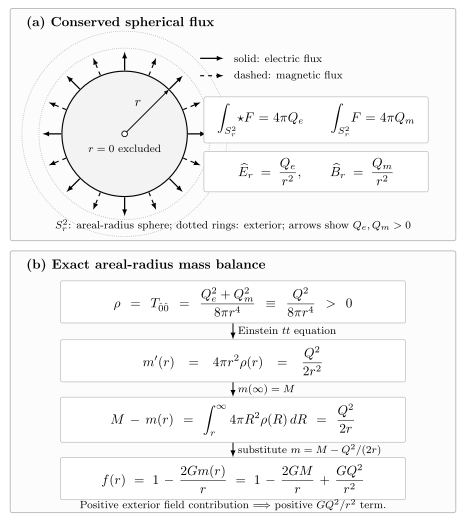
In the asymptotically flat $\Lambda=0$ specialization, electric and magnetic fluxes give radial fields proportional to $r^{-2}$ and positive energy density $\rho=Q^2/(8\pi r^4)$. The exact areal-radius mass balance is $M-m_{\rm MS}=Q^2/(2r)$, which yields $f=1-2GM/r+GQ^2/r^2$. Reversing either signed charge reverses the corresponding field arrows but leaves the metric unchanged. The displayed radial integral follows from the spherical Einstein equation; it is not a proper-volume integral on a static slice.

For $\Lambda=0$, the metric agrees after identifying Bičák’s geometrized parameters as $M_{\rm B}=GM$ and $Q_{\rm B}^2=GQ^2$ with the charged family in Bičák 2000, §3, Eqs. (9)–(10), printed pp. 31–32, Open PDF. Bičák displays the purely electric representative; the invariant Maxwell reduction above supplies the magnetic dual and shows why the geometry depends only on $Q_e^2+Q_m^2$.

Roots, horizons, and critical points

The norm of the additional Killing field is

$$K^2=-q=-f(r).$$

It is timelike where $f>0$, null where $f=0$, and spacelike where $f<0$. This is why “an additional local Killing field” is more accurate than “the solution is static everywhere.” In the advanced chart the determinant of the $(v,r)$ metric block is $-1$ at every finite positive root of $f$, whether the root is simple, double, or triple. The diagonal coefficient $f^{-1}$ is the singular object, not the invariant geometry.

A generic point on a Killing horizon still has $dr\ne0$ as a covector even though $(\nabla r)^2=0$. At a bifurcation two-sphere, by contrast, $K=0$ and $dr=0$. These isolated critical points are reached by smooth continuation of the Reissner–Nordström–(A)dS geometry; they do not form the constant-radius branch.

A positive multiple root $r_0$ obeys $f(r_0)=f'(r_0)=0$, hence

$$GQ^2=r_0^2(1-\Lambda r_0^2), \qquad GM=r_0\left(1-\frac23\Lambda r_0^2\right),$$

and

$$-\frac12f''(r_0)=2\Lambda-\frac1{r_0^2}.$$

For $\Lambda>0$, a triple root occurs at

$$r_0^2=\frac1{2\Lambda}, \qquad GQ^2=\frac1{4\Lambda}, \qquad GM=\frac{2r_0}{3}.$$

These algebraic facts locate degenerate Killing horizons. Their names and global roles require a chosen extension and asymptotic structure; Reissner–Nordström Horizons and Extensions supplies that global analysis.

Constant-radius product branches

If $r=r_0$ on an open set, the areal coordinate cannot be used. Put

$$S=E^2+B^2=\frac{Q^2}{r_0^4}.$$

The two factor equations from the theorem become

$$k_h=\Lambda-\frac{GQ^2}{r_0^4}, \qquad \frac1{r_0^2}=\Lambda+\frac{GQ^2}{r_0^4}.$$

Eliminating the field strength gives the branch polynomial and a useful curvature formula:

$$\Lambda r_0^4-r_0^2+GQ^2=0, \qquad k_h=2\Lambda-\frac1{r_0^2}.$$

The complete real, positive-radius classification is as follows.

Cosmological constant	Existence and factor geometry
$\Lambda>0$	Products exist exactly when $4\Lambda GQ^2\le1$. For nonzero charge below equality there are two radii: the smaller gives $\mathrm{AdS}_2\times S^2$, the larger gives charged $\mathrm{dS}_2\times S^2$ Nariai. Equality gives $\mathbb M^{1,1}\times S^2$. At $Q=0$, only $r_0^2=1/\Lambda$ survives as neutral Nariai.
$\Lambda=0$	Nonzero charge gives the unique $r_0^2=GQ^2$ Bertotti–Robinson geometry $\mathrm{AdS}_2\times S^2$ with equal curvature radii. There is no neutral finite-radius product.
$\Lambda<0$	Nonzero charge gives one positive radius and an $\mathrm{AdS}_2\times S^2$ product. There is no neutral spherical product.

For $\Lambda>0$, the two charged roots are

$$r_{0,\pm}^2 =\frac{1\pm\sqrt{1-4\Lambda GQ^2}}{2\Lambda}.$$

For $\Lambda<0$, the unique root is

$$r_0^2 =\frac{\sqrt{1+4|\Lambda|GQ^2}-1}{2|\Lambda|}.$$

The positive-$\Lambda$ and zero-$\Lambda$ factor equations and near-horizon limits are derived in Cardoso, Dias, and Lemos 2004, §III, Eqs. (13)–(29), printed pp. 3–6, Open PDF; their negative-$\Lambda$ construction is in Cardoso, Dias, and Lemos 2004, §IV.A–B, Eqs. (31), (33), and (37)–(39), printed pp. 7–9. The flat-factor solution is commonly grouped with the Plebański–Hacyan geometries; see Podolský and Ortaggio 2003, §3.1, Eq. (25), printed p. 5, and Table 2, printed pp. 7–8, Open PDF.

The dimensionless positive-$\Lambda$ curve makes the two roots and their merger especially transparent. Read the sign of $k_h$ on either side of the maximum, then follow the lower strip: the product geometry is obtained only after a near-horizon scaling.

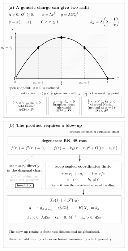
Top: for $x=\Lambda r_0^2$ and $y=\Lambda GQ^2$, the exact relation $y=x(1-x)$ gives two radii when $0<y<1/4$. The smaller root has $k_h<0$ and an $\mathrm{AdS}_2$ factor; the larger has $k_h>0$ and a $\mathrm{dS}_2$ factor. They meet at the ultracold point $x=1/2$, $y=1/4$, where $k_h=0$; $x=0$ is excluded, while $x=1$ is neutral Nariai. Bottom: the equations are exact and the flow is schematic. A correlated near-horizon blow-up retains $X_2(k_h)\times S^2(r_0)$, whereas direct substitution at the degenerate Reissner–Nordström–de Sitter root produces no four-dimensional product geometry.

For every product radius, the multiple-root equations above select a corresponding degenerate Reissner–Nordström–(A)dS parameter pair. That correspondence does not identify the two four-dimensional neighborhoods. The product is obtained by magnifying a shrinking near-horizon region while rescaling time; direct substitution $r=r_0$ into the varying-radius metric produces a degenerate pullback, not the product solution. Near-Horizon Scaling Limits develops this limiting operation.

What is and is not fixed by the metric

The metric depends on the electromagnetic field only through $Q^2=Q_e^2+Q_m^2$. It therefore cannot determine the signs of the charges or the electric–magnetic duality angle. Two fields with the same $Q^2$ can source the same metric without being the same metric–field solution.

Ordinary Maxwell gauge equivalence compares potentials with the same two-form $F$. A constant duality rotation changes $F$ and is an extra equivalence only if one explicitly chooses to quotient the source-free theory by duality. A spacetime-dependent duality angle does not preserve the source-free equations in general. These distinctions matter whenever one classifies the complete solution rather than only its line element.

How the conclusion can fail

Keep the advanced line element, but allow its parameters to vary along $v$:

$$f(v,r)=1-\frac{2GM(v)}r +\frac{G[Q_e(v)^2+Q_m(v)^2]}{r^2} -\frac{\Lambda r^2}{3}$$

and pair it with

$$F=-\frac{Q_e(v)}{r^2}\,dv\wedge dr+Q_m(v)\omega.$$

This is a compact adverse test. Define the Einstein–Maxwell–Lambda residual by

$$\mathcal E_{\mu\nu} =G_{\mu\nu}+\Lambda g_{\mu\nu} -8\pi G T^{\rm EM}_{\mu\nu}.$$

Its null component is

$$\mathcal E_{vv} =\frac{2G}{r^3} \left(r\dot M-Q_e\dot Q_e-Q_m\dot Q_m\right).$$

With constant charges and $\dot M\ne0$, this is Vaidya-type null matter, so electrovac has been abandoned. With varying electric charge, $d{*F}=0$ fails unless an electric current is supplied; varying magnetic charge violates $dF=0$ unless magnetic current is added. Nevertheless the scalar curvature remains $R=4\Lambda$, showing why a scalar-curvature check alone cannot establish the theorem.

Other failures are equally diagnostic. Charged matter, a time-dependent scalar, or a null fluid can add quotient stress that is not proportional to $h_{ab}$. Merely setting one coordinate flux component to zero is weaker than the pure-trace condition needed by the Killing proof. When Birkhoff’s Conclusion Fails compares these hypothesis changes systematically.

Common pitfalls

Reading Birkhoff as global staticity. The theorem supplies a local Killing field. Its norm changes sign with $f$, and no local calculation alone identifies an event horizon or a preferred maximal extension.

Confusing $q=0$ with $dr=0$. At an ordinary Killing horizon, the areal-radius gradient is null but generally nonzero. The constant-radius branch requires $dr=0$ throughout an open set.

Dropping the orientation-dependent electric sign. With $\epsilon_g=\epsilon_h\wedge r^2\omega$, one has $*\epsilon_h=-r^2\omega$. The minus sign in $F=-Q_e\epsilon_h/r^2+Q_m\omega$ is what makes the electric flux equal $+Q_e$.

Giving the charge term the wrong sign. Maxwell energy density is positive. The exterior contribution lowers the mass enclosed by a finite sphere and therefore produces $+GQ^2/r^2$ in $f$.

Identifying a multiple-root metric with its product limit. A degenerate horizon and its near-horizon product share parameters and limiting curvature data, but not an unscaled neighborhood. The coordinate blow-up is essential.

Calling $M$ an ADM mass without an asymptotic end. Locally, $M$ is the invariant integration constant in the mass balance. ADM terminology requires additional global boundary conditions and normalization.

Classifying only the metric. The metric fixes $Q^2$, not $Q_e$, $Q_m$, their signs, or the two-form. Gauge equivalence and duality equivalence are different statements.

Exercises

1. Recover the charges from the Hodge star

Using the stated orientation and Hodge identities, verify $*F$ and evaluate both flux integrals. What changes if the quotient orientation is reversed while the four-dimensional orientation is held fixed?

Solution

Linearity and the two Hodge identities give

$$*F=-\frac{Q_e}{r^2}(-r^2\omega) +Q_m\frac{\epsilon_h}{r^2} =Q_e\omega+\frac{Q_m}{r^2}\epsilon_h.$$

The pullback of $\epsilon_h$ to a symmetry sphere vanishes, while $\int_{S^2}\omega=4\pi$. Hence

$$\frac1{4\pi}\int_{S^2}*F=Q_e, \qquad \frac1{4\pi}\int_{S^2}F=Q_m.$$

Holding $\epsilon_g$ fixed while reversing $\epsilon_h$ also reverses the compatible sphere orientation. Both signed flux labels change with the corresponding orientation convention, while $Q^2$, the stress tensor, and the metric do not.

2. Derive the stress blocks and the Killing field

In an adapted orthonormal frame, take radial field magnitudes $E=Q_e/r^2$ and $B=Q_m/r^2$. Show that the mixed stress tensor is $\rho\operatorname{diag}(-1,-1,1,1)$, then use the trace-free quotient Einstein equation to prove that $K_a=\epsilon_a{}^b\nabla_b r$ is Killing.

Solution

The Maxwell energy density is $(E^2+B^2)/(8\pi)=Q^2/(8\pi r^4)$. A radial electromagnetic field has tension $-\rho$ parallel to the field and pressure $+\rho$ in each transverse direction. Thus

$$T^{\hat\mu}{}_{\hat\nu} =\rho\operatorname{diag}(-1,-1,1,1),$$

which is equivalent to $T_{ab}=-\rho h_{ab}$ on the quotient. Its trace-free part vanishes, so Einstein’s equation gives

$$\nabla_a\nabla_b r=\frac12(\Box_h r)h_{ab}.$$

Now

$$\nabla_{(a}K_{b)} =\epsilon_{(b}{}^c\nabla_{a)}\nabla_c r =\frac12(\Box_h r)\epsilon_{(b}{}^c h_{a)c}=0,$$

because the last tensor is the symmetrization of an antisymmetric volume form. Since $K(r)=0$, this quotient Killing field also preserves the sphere factor and is Killing for the full metric.

3. Find the conserved electrovac mass

Starting from $m_{\rm MS}=r(1-q)/(2G)$, the Hessian equation, and the angular Einstein equation, derive $\nabla_am_{\rm MS}$ and prove that $M$ is constant. Check the limits $Q=0$ and $\Lambda=0$.

Solution

The Hessian equation gives

$$\nabla_aq =2\nabla_a\nabla_b r\,\nabla^b r =(\Box_h r)\nabla_a r.$$

Therefore

$$\begin{aligned} \nabla_a m_{\rm MS} &=\frac1{2G}\left[(1-q)\nabla_a r-r\nabla_aq\right]\\ &=\frac1{2G}(1-q-r\Box_h r)\nabla_a r\\ &=\left(\frac{\Lambda r^2}{2G}+\frac{Q^2}{2r^2}\right)\nabla_a r. \end{aligned}$$

Since $Q$ and $\Lambda$ are constant,

$$\nabla_a\left(m_{\rm MS}+\frac{Q^2}{2r}-\frac{\Lambda r^3}{6G}\right)=0.$$

The bracket is $M$. When $Q=0$, this is the cosmologically subtracted Kottler mass. When $\Lambda=0$, it is the Reissner–Nordström mass $m_{\rm MS}+Q^2/(2r)$.

4. Classify every constant-radius product

Solve $\Lambda r_0^4-r_0^2+GQ^2=0$ for each sign of $\Lambda$. Use $k_h=2\Lambda-r_0^{-2}$ to identify the quotient factor, including the neutral endpoints.

Solution

For $\Lambda>0$, set $x=r_0^2$. The discriminant is $1-4\Lambda GQ^2$, so positive roots exist exactly when $4\Lambda GQ^2\le1$:

$$x_\pm=\frac{1\pm\sqrt{1-4\Lambda GQ^2}}{2\Lambda}.$$

For nonzero subcritical charge, $x_-<1/(2\Lambda)$ gives $k_h<0$ and hence $\mathrm{AdS}_2$, while $x_+>1/(2\Lambda)$ gives $k_h>0$ and hence $\mathrm{dS}_2$. At equality, $k_h=0$. When $Q=0$, $x_-=0$ is not a positive-radius geometry; $x_+=1/\Lambda$ is neutral Nariai.

For $\Lambda=0$, $x=GQ^2$, which is positive only for nonzero charge, and $k_h=-1/x$: Bertotti–Robinson. For $\Lambda=-|\Lambda|<0$,

$$x=\frac{\sqrt{1+4|\Lambda|GQ^2}-1}{2|\Lambda|}$$

is the only positive root when $Q\ne0$, and $k_h<0$. Setting $Q=0$ leaves no positive finite root for $\Lambda\le0$.

5. Factorize extremal Reissner–Nordström

Let $\Lambda=0$, $M>0$, and $GQ^2=(GM)^2$. Factorize $f$, locate its repeated positive root, and explain why Bertotti–Robinson is not obtained by simply setting $r$ equal to that root.

Solution

The extremal relation gives

$$f(r)=1-\frac{2GM}{r}+\frac{(GM)^2}{r^2} =\left(1-\frac{GM}{r}\right)^2.$$

Because $M>0$, the repeated root $r_0=GM$ lies in the physical region $r>0$. If $M=0$, the charge also vanishes and there is no positive root; if $M<0$, the algebraic root is negative. At $r=r_0$, direct restriction removes the radial direction and makes the static-coordinate pullback degenerate. Bertotti–Robinson instead follows from a scaling such as $r=r_0+\varepsilon R$ and $t=T/\varepsilon$, followed by $\varepsilon\to0$, which retains a nondegenerate two-dimensional throat.

Continue through the subject

• The Reissner–Nordström Solution develops the charged solution through its metric, field, curvature, and gauge patches.
• Reissner–Nordström Horizons and Extensions classifies roots and constructs the global analytic extensions.
• Nariai and Bertotti–Robinson Geometries studies the product solutions in their own coordinates.
• Near-Horizon Scaling Limits explains the controlled blow-ups that connect degenerate horizons to product throats.
• When Birkhoff’s Conclusion Fails tests matter flux, scalar fields, symmetry inheritance, and modified field equations.

References

• Bičák, Jiří. “Selected Solutions of Einstein’s Field Equations: Their Role in General Relativity and Astrophysics.” In Einstein’s Field Equations and Their Physical Implications, edited by Bernd G. Schmidt, Lecture Notes in Physics 540, 1–126. Berlin: Springer, 2000. doi:10.1007/3-540-46580-4_1; arXiv:gr-qc/0004016v1, Open PDF.
• Cardoso, Vitor, Óscar J. C. Dias, and José P. S. Lemos. “Nariai, Bertotti–Robinson and Anti-Nariai Solutions in Higher Dimensions.” Physical Review D 70 (2004): 024002. doi:10.1103/PhysRevD.70.024002; arXiv:hep-th/0401192v2, Open PDF.
• Hayward, Sean A. “Gravitational Energy in Spherical Symmetry.” Physical Review D 53 (1996): 1938–1949. doi:10.1103/PhysRevD.53.1938; arXiv:gr-qc/9408002v2, Open PDF.
• Podolský, Jiří, and Marcello Ortaggio. “Explicit Kundt Type II and N Solutions as Gravitational Waves in Various Type D and O Universes.” Classical and Quantum Gravity 20 (2003): 1685–1701. doi:10.1088/0264-9381/20/9/307; arXiv:gr-qc/0212073v2, Open PDF.
• Stephani, Hans, Dietrich Kramer, Malcolm MacCallum, Cornelius Hoenselaers, and Eduard Herlt. Exact Solutions of Einstein’s Field Equations. 2nd ed. Cambridge: Cambridge University Press, 2003. doi:10.1017/CBO9780511535185.