Stationary and Axial Killing Geometry

A stationary axisymmetric spacetime has two continuous symmetries: time translation and rotation. The invariant data are the two Killing fields, their group action, and their inner products—not whether a chosen metric happens to contain a $dt\,d\phi$ term. The central test is local and coordinate-free: a chosen stationary Killing field $k$ defines staticity where it is timelike only if $k^\flat\wedge dk^\flat=0$, equivalently if its twist vanishes. This page develops that test together with the invariants that distinguish axes, Killing horizons, and stationary-limit surfaces, then checks the whole toolkit on Minkowski, Schwarzschild, and Kerr spacetimes.

Required background. Killing Fields and Isometry Groups supplies Killing flows and fixed sets; The Einstein Equation supplies the field equations used on the next page to constrain the orbit geometry. The tests developed here are kinematical, so no field equation is needed until the circularity argument.

Helpful background. The Riemann Curvature Tensor supports invariant checks; Formulations of General Relativity supplies reduced and initial-value viewpoints; Causality and Global Structure supports the distinction between local Killing data and global stationarity.

The stationary and axial actions

Let $\xi$ generate an $\mathbb R$ action and let $\eta$ generate an effective $U(1)$ action on the spacetime region under study. “Effective” means that no nonidentity rotation acts trivially everywhere. In the standard asymptotically flat black-hole setting, $\xi$ is the globally selected symmetry generator that is timelike near a chosen asymptotic end and is normalized there as the unit time translation. The generic orbit of $\eta$ is closed, and we normalize its parameter to have period $2\pi$. In the usual four-dimensional meaning of axisymmetry, the action has a nonempty codimension-two fixed set—the axis—on which $\eta=0$.

The usual stationary-axisymmetric action is Abelian:

$$\mathcal L_\xi g=0, \qquad \mathcal L_\eta g=0, \qquad [\xi,\eta]=0.$$

Locally, away from fixed points, commutation permits adapted coordinates $(t,\phi,x^1,x^2)$ with $\xi=\partial_t$, $\eta=\partial_\phi$, and $\phi\sim\phi+2\pi$. These coordinates expose the symmetries, but they do not define them. In particular, replacing $\xi$ by $\xi+\Omega\eta$ changes which Killing flow is called “time translation.” The asymptotic normalization determines which choice has the intended physical meaning. A Killing field may also be timelike on one local patch without extending to the selected global stationary action; those are different claims.

These definitions, including the distinction between stationary, static, and axial actions, are developed in Chruściel, Costa, and Heusler 2012, §§3.1–3.2.3, printed pp. 12–14, Open PDF.

The two-Killing Gram matrix

Package the inner products of the generators into

$$\lambda_{AB}=g(K_A,K_B), \qquad (K_0,K_1)=(\xi,\eta).$$

On the regular set where $\xi$ and $\eta$ are independent and a local quotient exists, the group orbits are two-dimensional. Because both generators preserve the metric and commute, every entry of $\lambda_{AB}$ is constant along both flows and descends to the local orbit space

$$\mathcal Q=\mathcal U/(\mathbb R\times U(1)).$$

Axes become boundary pieces of the completed quotient rather than points of this regular rank-two set. Where a group orbit is a timelike two-surface, define the invariant function

$$\rho^2\equiv-\det\lambda =g(\xi,\eta)^2-g(\xi,\xi)g(\eta,\eta)\geq0.$$

Under a constant change of Killing basis $K'_A=A_A{}^B K_B$,

$$\lambda'=A\lambda A^{\mathsf T}, \qquad \det\lambda'=(\det A)^2\det\lambda.$$

Thus the zero set of $\det\lambda$ is basis-independent, although $\rho$ rescales by $|\det A|$. It becomes a useful Weyl radial coordinate only after additional field-equation, circularity, and regularity hypotheses; at this stage it is merely a scalar on the quotient. Physical normalizations at infinity and around the axis also restrict which basis changes preserve the intended $\mathbb R\times U(1)$ action.

When $\det\lambda=0$, the Gram block has a kernel: some coefficient vector $v^A$ makes $v^A K_A$ orthogonal to both symmetry generators. The kernel, not the determinant alone, identifies what has degenerated. On an ordinary axis the kernel is generated by $\eta$; on a regular rotating Killing horizon it is generated by $K_H=\xi+\Omega_H\eta$. Here a Killing horizon is a null hypersurface to which a Killing field is normal. The determinant condition alone does not prove that a candidate surface is smooth, null, or a horizon.

A stationary-limit surface is instead a locus where the selected stationary field becomes null, $g(\xi,\xi)=0$. If at such a point $b=g(\xi,\eta)\ne0$, then

$$\lambda= \begin{pmatrix}0&b\\ b&g(\eta,\eta)\end{pmatrix}, \qquad \det\lambda=-b^2<0.$$

Thus a null basis vector need not lie in the kernel: the Killing block can remain nondegenerate.

Staticity and twist

Write $k^\flat=g(k,\mathord\cdot)$. On any region where $k\ne0$, the Killing field is hypersurface orthogonal precisely when the three-planes annihilated by $k^\flat$ integrate to hypersurfaces. Frobenius’ theorem gives three equivalent tests:

$$k^\flat\wedge dk^\flat=0, \qquad k_{[\mu}\nabla_\nu k_{\rho]}=0, \qquad \omega_\mu(k)=0,$$

where

$$\omega_\mu(k)=\epsilon_{\mu\nu\rho\sigma} k^\nu\nabla^\rho k^\sigma$$

is the twist one-form. A particular stationary field is locally static wherever it is timelike and passes this test. A spacetime region is static if it admits such a timelike Killing field. A global static product additionally requires global hypotheses; the local Frobenius condition alone does not supply them. This local criterion and its distinction from global staticity are stated in Chruściel, Costa, and Heusler 2012, §3.1, printed pp. 12–13, Open PDF.

Normalization cannot change the answer. For any nonzero constant $c$,

$$(ck)^\flat\wedge d(ck)^\flat =c^2 k^\flat\wedge dk^\flat.$$

Normalization matters for numerical quantities such as energy, angular velocity, or surface gravity, but not for whether twist vanishes. Likewise, a time-independent diagonal chart adapted to $k=\partial_t$ is sufficient for hypersurface orthogonality, because $k^\flat=g_{tt}\,dt$ immediately gives $k^\flat\wedge dk^\flat=0$. Diagonality is not necessary: a different coordinate chart can hide staticity behind cross terms.

It helps to keep five notions separate:

Notion	Invariant question	What does not decide it by itself?
Stationary	Is there a selected $\mathbb R$ isometry whose generator has the required timelike domain—near the chosen asymptotic end in the black-hole setting?	A Killing field that is timelike only on an unrelated local patch
Static	Does the region admit a timelike, hypersurface-orthogonal Killing field?	The presence or absence of one displayed $g_{t\phi}$ term
Axisymmetric	Is there an effective periodic isometry with a nonempty fixed set?	Merely using a coordinate named $\phi$
Circular	Are the two-surfaces orthogonal to the group orbits integrable?	Staticity of one generator, or commutation alone
Regular axis	Does the fixed set have the correct local geometry and differentiability?	The equation $g(\eta,\eta)=0$ alone

The word “rotating” is correspondingly context-dependent. It may refer to nonzero twist of a chosen stationary field, nonzero ADM or Komar angular momentum, frame dragging, matter vorticity, or simply rotating coordinates. A careful argument names the diagnostic it uses.

Three examples that separate the concepts

Minkowski spacetime in a rotating chart

Begin with inertial cylindrical coordinates:

$$ds^2=-dT^2+dR^2+R^2d\Phi^2+dZ^2.$$

For $\xi_0=\partial_T$ and $\eta=\partial_\Phi$,

$$\lambda=\begin{pmatrix}-1&0\\0&R^2\end{pmatrix}, \qquad \rho^2=R^2.$$

Now set $T=t$ and $\Phi=\phi+\Omega t$. The same flat metric becomes

$$ds^2=-(1-\Omega^2R^2)dt^2 +2\Omega R^2dt\,d\phi +R^2d\phi^2+dR^2+dZ^2.$$

The integral curves of $K=\partial_t=\xi_0+\Omega\eta$ are helices: at fixed $(R,\phi,Z)$ they rotate with inertial angular velocity $\Omega$. Their squared tangent norm is

$$K^2=-1+\Omega^2R^2.$$

For $\Omega\ne0$, $K$ is timelike precisely for $R<|\Omega|^{-1}$, null on the light cylinder $R_L=|\Omega|^{-1}$, and spacelike outside it. Only the inner curves can therefore be worldlines of observers following this coordinate flow. For $\Omega=0$, $K$ reduces to the inertial generator and is timelike everywhere. Its dual and Frobenius three-form are

$$\begin{aligned} K^\flat&=-(1-\Omega^2R^2)dt+\Omega R^2d\phi,\\ K^\flat\wedge dK^\flat &=-2\Omega R\,dt\wedge dR\wedge d\phi. \end{aligned}$$

So the helical field twists away from the axis when $\Omega\ne0$. Nevertheless, the inertial generator $\xi_0=K-\Omega\eta$ has $\xi_0^\flat=-dt$ and zero twist. Moreover,

$$\det\lambda_{(K,\eta)}=-R^2, \qquad g^{RR}=1.$$

The Killing block is therefore nondegenerate at $R_L$, and the light-cylinder hypersurface has a spacelike normal, so it is timelike—not a Killing horizon or a metric singularity. The cross term and the behavior of $K$ diagnose the chosen rotating flow, not intrinsic nonstaticity of Minkowski spacetime.

The figure makes this change of generator visible. Read the causal-cone panels from left to right: the inertial field stays vertical while the helical field passes from timelike through null to spacelike.

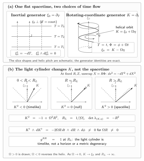
Same flat spacetime, different Killing flows. Under $T=t$ and $\Phi=\phi+\Omega t$, $K=\partial_t=\xi_0+\Omega\eta$ has $K^2=-1+\Omega^2R^2$ and a nonzero Frobenius three-form away from the axis, while $\xi_0=K-\Omega\eta$ has dual $-dt$ and zero twist. The light cylinder changes the causal character of $K$ but is neither a horizon nor a metric degeneracy because $\det\lambda_{(K,\eta)}=-R^2$ is nonzero there. Equations and radii are exact; the slice and helix layout is schematic. The drawing uses $\Omega>0$; changing its sign reverses the helix.

Schwarzschild exterior

For the Schwarzschild exterior, write $m=GM$ and $f=1-2m/r$. With $\xi=\partial_t$ and $\eta=\partial_\phi$,

$$\lambda=\begin{pmatrix} -f&0\\ 0&r^2\sin^2\theta \end{pmatrix}, \qquad \rho^2=fr^2\sin^2\theta.$$

Since $\xi^\flat=-f\,dt$, the exterior is static. At $\sin\theta=0$ the axial field vanishes and the Gram kernel is generated by $\eta$. On the regular extension of $f=0$, away from the axis and bifurcation two-sphere, the nonzero null horizon generator is instead $\xi$. The same determinant condition therefore describes two geometrically different boundary pieces.

Kerr: horizon, axis, and stationary limit

Consider the four-dimensional asymptotically flat vacuum Kerr metric in Boyer–Lindquist coordinates. Retain $m=GM$ and define $a=J/M$ in $c=1$ units. Thus $m$ and $a$ are lengths, $a/m=J/(GM^2)$, and $\Omega_H$ has inverse-length dimension. Assume $m>0$ and $|a|<m$ for the horizon comparison, and define

$$r_\pm=m\pm\sqrt{m^2-a^2},$$ $$\Sigma=r^2+a^2\cos^2\theta, \qquad \Delta=(r-r_+)(r-r_-)=r^2-2mr+a^2.$$

The exterior Boyer–Lindquist chart has $r>r_+$, $0<\theta<\pi$, and $\Sigma>0$. Axis and horizon statements below use finite limits of the invariant Killing inner products and their regular extensions, because the Boyer–Lindquist coordinates themselves do not cover those loci regularly. Here $r_+$ is the outer horizon radius. For $0<|a|<m$, $r_-$ is the inner Cauchy and Killing-horizon radius; at the Schwarzschild endpoint $a=0$, the formal root $r_-=0$ is the central curvature singularity, not a horizon. At $|a|=m$, the roots merge at the degenerate horizon $r=m$. When $|a|>m$, $\Delta$ has no real roots and Kerr has no black-hole horizon.

Direct evaluation of the $(t,\phi)$ block gives the exact identity

$$\det\lambda=-\Delta\sin^2\theta.$$

On a regular axis away from a horizon, the kernel is generated by $\eta$. On a horizon $r=r_+$ away from the axis, it is generated by

$$K_H=\xi+\Omega_H\eta, \qquad \Omega_H=\frac{a}{r_+^2+a^2}.$$

At a horizon–axis corner the coefficient matrix vanishes, so its coefficient-space kernel is two-dimensional. This algebra alone does not determine which spacetime Killing vectors vanish. At a pole of a future or past horizon branch away from the bifurcation surface, $\eta=0$ while $K_H$ is nonzero and null; at a bifurcation-axis point, $K_H$ vanishes as well. Coefficient-space kernel, tangent-space fixed set, and null generator must therefore be distinguished.

The stationary-limit surface instead satisfies $g_{tt}=0$, or $2mr=\Sigma$. Substitution gives

$$\Delta=a^2\sin^2\theta, \qquad \det\lambda=-a^2\sin^4\theta.$$

Thus a generic stationary-limit point with $a\sin\theta\ne0$ has an invertible Killing block. It is not an axis or a Killing horizon merely because $\xi$ becomes null there. With the site orientation $\epsilon_{tr\theta\phi}=+\sqrt{-g}$ in the displayed coordinate ordering and the additive gauge fixed by $\chi\to0$ at the selected asymptotically flat end, the vacuum twist potential defined by $d\chi=\omega(\xi)$ is

$$\chi=-\frac{2ma\cos\theta}{\Sigma},$$

and direct differentiation gives

$$d\chi= \frac{4mar\cos\theta}{\Sigma^2}\,dr +\frac{2ma\left(r^2-a^2\cos^2\theta\right)\sin\theta}{\Sigma^2}\,d\theta.$$

Substitution of the Boyer–Lindquist metric into the twist definition produces exactly these two nonzero components. Hence $\chi$ is nonconstant when $ma\ne0$, and the asymptotically normalized $\xi$ is not hypersurface orthogonal. Nor can a constant co-rotating combination remain an asymptotic time translation. For fixed $\Omega$,

$$\begin{aligned} g(\xi+\Omega\eta,\xi+\Omega\eta) ={}&-1+\Omega^2(r^2+a^2)\sin^2\theta\\ &+\frac{2mr}{\Sigma} \left(1-a\Omega\sin^2\theta\right)^2. \end{aligned}$$

The last term is $O(r^{-1})$ at fixed angle, so every constant $\Omega\ne0$ makes the combination spacelike sufficiently far out away from the axis. The metric, horizon generator, and stationary-limit geometry are reviewed in Bičák 2000, §4.1, printed pp. 42–45, Open PDF.

The exact meridional comparison is shown on Kerr Domains, Horizons, and Extensions. For a complementary orbit-space picture of how the axis and horizon pieces meet, see the Schwarzschild calibration, which includes the chapter’s axis-interval diagram.

Testing an ordinary axis

Let

$$\mathcal A=\{p:\eta_p=0\}, \qquad X=g(\eta,\eta).$$

Approach an ordinary axis through a normal neighborhood where $X>0$. If $\ell$ is proper distance in the transverse two-plane and the axial orbits have period $2\pi$, smooth polar behavior gives

$$X=\ell^2+O(\ell^4), \qquad \nabla_\mu X\nabla^\mu X=4\ell^2+O(\ell^4).$$

Therefore elementary flatness requires

$$\lim_{\substack{p\to\mathcal A\\X(p)>0}} \frac{\nabla_\mu X\nabla^\mu X}{4X}=1.$$

The fixed-set qualifier matters: $X=0$ can also occur where a nonzero axial generator becomes null, and such a locus is not an axis. The normalization is essential as well: rescaling $\eta$ by a constant rescales the limit by its square. For $\alpha>0$, consider the transverse cone

$$ds^2=dR^2+\alpha^2R^2d\phi^2, \qquad \phi\sim\phi+2\pi,$$

Here $X=\alpha^2R^2$, so the limit is $\alpha^2$. The circumference-to-radius ratio is $2\pi\alpha$, and the signed conical deficit is $2\pi(1-\alpha)$.

Elementary flatness rules out this conical defect, but it is not by itself a complete smoothness theorem. One must also check differentiability of the metric and tensor fields in regular local Cartesian coordinates. The inspected abstract distinguishes these regularity questions in Wilson and Clarke 1996, abstract and article metadata.

These conditions become boundary data for the later reduction. The chapter now proceeds in logical order: circularity and orthogonal transitivity justify meridional surfaces; the Weyl–Papapetrou orbit space supplies canonical reduced coordinates; twist and Ernst potentials encode the vacuum equations; relativistic multipoles read asymptotic structure; and ergoregions, Killing horizons, and axes interpret the quotient boundary.

Common pitfalls

Reading physics from one chart. A $dt\,d\phi$ term says that the displayed time flow is not orthogonal to the displayed time slices. It does not, without a Killing-field and twist analysis, prove that the spacetime is intrinsically nonstatic.

Treating every zero determinant alike. The scalar $\det\lambda$ locates degeneracy of the group orbit, but its kernel distinguishes an axis generator from a horizon generator. At a generic Kerr stationary limit, the determinant does not vanish.

Calling every null-Killing locus a horizon. A selected Killing field can become null on a timelike hypersurface, as $K$ does at the rotating-Minkowski light cylinder. A Killing horizon must itself be null and have a Killing field as its normal.

Equating elementary flatness with full regularity. The scalar limit detects a conical defect after the axial period is fixed. Smooth extension of all fields across the axis requires additional differentiability checks.

Exercises

1. Diagonal form and normalization

Suppose a stationary chart has $k=\partial_t$ and $g_{ti}=0$ for every spatial coordinate $x^i$. Prove that $k$ is hypersurface orthogonal. Then show that $k\mapsto ck$, for constant $c\ne0$, cannot change this conclusion.

Solution

The metric dual is $k^\flat=g_{tt}\,dt$. Therefore

$$\begin{aligned} dk^\flat&=dg_{tt}\wedge dt,\\ k^\flat\wedge dk^\flat &=g_{tt}\,dt\wedge dg_{tt}\wedge dt=0. \end{aligned}$$

Frobenius therefore makes $k$ hypersurface orthogonal wherever it is nonzero. For constant $c$, $(ck)^\flat\wedge d(ck)^\flat=c^2k^\flat\wedge dk^\flat$, so zero remains zero and nonzero remains nonzero.

2. The helical field in flat spacetime

Derive the rotating Minkowski metric above, compute $K^\flat\wedge dK^\flat$ for $K=\partial_t$, and identify its light cylinder and the static generator.

Solution

From $d\Phi=d\phi+\Omega dt$,

$$R^2d\Phi^2=R^2d\phi^2+2\Omega R^2dt\,d\phi+\Omega^2R^2dt^2,$$

which yields the displayed metric. Since $K^2=-1+\Omega^2R^2$, $K$ is null at $R=|\Omega|^{-1}$, the light cylinder. Differentiating

$$K^\flat=-(1-\Omega^2R^2)dt+\Omega R^2d\phi$$

and taking the wedge product gives

$$K^\flat\wedge dK^\flat=-2\Omega R\,dt\wedge dR\wedge d\phi.$$

The inertial generator is $\partial_T=\partial_t-\Omega\partial_\phi$; its dual is $-dt$, so it is hypersurface orthogonal. In the rotating basis, $\det\lambda_{(K,\eta)}=-R^2$, which is nonzero at the light cylinder. Since $g^{RR}=1$, that cylinder has a spacelike normal and is timelike rather than a Killing horizon.

3. Three degeneracy tests in Kerr

Using the Boyer–Lindquist Killing block, verify $\det\lambda=-\Delta\sin^2\theta$. Identify the kernel on an ordinary axis and on the outer horizon, and show that a generic stationary-limit point has no kernel.

Solution

The needed components are

$$g_{tt}=-\left(1-\frac{2mr}{\Sigma}\right), \qquad g_{t\phi}=-\frac{2mar\sin^2\theta}{\Sigma},$$ $$g_{\phi\phi}=\sin^2\theta\left( r^2+a^2+\frac{2ma^2r\sin^2\theta}{\Sigma} \right).$$

Substitution into $g_{tt}g_{\phi\phi}-g_{t\phi}^2$ simplifies to $-\Delta\sin^2\theta$. On $\sin\theta=0$ with $\Delta\ne0$, the kernel is $(0,1)$, corresponding to $\eta$.

On a horizon $r=r_H$, use $\Delta(r_H)=0$ and $2mr_H=r_H^2+a^2\equiv A_H$. The Killing block becomes

$$\lambda_H= \frac{\sin^2\theta}{\Sigma_H} \begin{pmatrix} a^2&-aA_H\\ -aA_H&A_H^2 \end{pmatrix}.$$

Multiplying by $(1,a/A_H)^{\mathsf T}$ gives zero in both rows. Thus the off-axis horizon kernel is $(1,\Omega_H)$ with $\Omega_H=a/A_H$, corresponding to $K_H=\xi+\Omega_H\eta$. At $g_{tt}=0$, the relation $2mr=\Sigma$ gives $\det\lambda=-a^2\sin^4\theta$, which is nonzero when $a\sin\theta\ne0$.

4. Detecting a conical defect

For $\alpha>0$ and $ds^2=dR^2+\alpha^2R^2d\phi^2$ with $\phi\sim\phi+2\pi$, evaluate the elementary-flatness scalar and derive the signed deficit angle.

Solution

Here $X=\eta^2=\alpha^2R^2$ and $\nabla_R X=2\alpha^2R$. Hence

$$\frac{(\nabla X)^2}{4X} =\frac{4\alpha^4R^2}{4\alpha^2R^2} =\alpha^2.$$

A circle of proper radius $R$ has circumference $2\pi\alpha R$, so the signed deficit relative to a smooth plane is $2\pi(1-\alpha)$; negative values describe an angular excess. The $2\pi$-periodic chart is elementary-flat only when $\alpha=1$.

5. A null generator without a Gram kernel

At a stationary-limit point suppose

$$\lambda= \begin{pmatrix}0&b\\b&c\end{pmatrix}, \qquad b\ne0.$$

Show that $\xi$ is null but is not in the kernel, find $\det\lambda$, and explain why the zero set of the determinant is unchanged by any constant invertible Killing-basis transformation.

Solution

The coefficient vector of $\xi$ is $e_0=(1,0)^{\mathsf T}$. Although $e_0^{\mathsf T}\lambda e_0=0$, one has

$$\lambda e_0= \begin{pmatrix}0\\b\end{pmatrix}\ne0.$$

Thus $\xi$ is null but not orthogonal to the whole Killing plane. Moreover,

$$\det\lambda=-b^2<0,$$

so the plane is nondegenerate and Lorentzian. Under $K'_A=A_A{}^B K_B$,

$$\det\lambda'=(\det A)^2\det\lambda.$$

For constant invertible $A$, the multiplier is nonzero; hence the determinant vanishes at exactly the same spacetime points, even though its numerical normalization changes.

References

• Bičák, Jiří. “Selected Solutions of Einstein’s Field Equations: Their Role in General Relativity and Astrophysics.” In Einstein’s Field Equations and Their Physical Implications: Selected Essays in Honour of Jürgen Ehlers, edited by Bernd G. Schmidt, 1–126. Lecture Notes in Physics 540. Berlin and Heidelberg: Springer, 2000. DOI. Open PDF.
• Chruściel, Piotr T., João Lopes Costa, and Markus Heusler. “Stationary Black Holes: Uniqueness and Beyond.” Living Reviews in Relativity 15, 7 (2012). DOI. Open PDF.
• Wilson, J. P., and C. J. S. Clarke. “‘Elementary Flatness’ on a Symmetry Axis.” Classical and Quantum Gravity 13 (1996): 2007–2027. DOI. Southampton abstract and metadata.