Relativistic Multipole Moments

Relativistic multipole moments describe the stationary gravitational field at one chosen asymptotically flat end. They are not simply the coefficients of an arbitrary $1/r$ expansion: radial gauge changes alter those coefficients, translations mix multipole orders, and rotations mix components within a fixed order. The cure is to normalize the stationary Killing field, fix the twist gauge and an origin, and then use either the coordinate-independent Geroch–Hansen construction or an asymptotically Cartesian, mass-centered expansion. This page develops both routes and checks them on Kerr and the inequivalent Zipoy–Voorhees family.

Required background. Killing Fields and Isometry Groups supplies the stationary quotient; The Einstein Equation supplies the vacuum equations that control the asymptotic data.

Helpful background. The Riemann Curvature Tensor supports the conformal-curvature correction; Formulations of General Relativity supplies asymptotic decompositions; Causality and Global Structure supplies the assumptions behind a selected asymptotic end.

Which multipoles are being defined?

The moments here are stationary field multipoles of a vacuum exterior near spatial infinity. They encode the asymptotic geometry generated by matter and by the gravitational field together. They are different objects from material-source integrals, the time-dependent source and radiative moments used in wave generation, and the quasi-local moments of a finite horizon cross-section. Those notions agree only in special limits or after a theorem supplies a bridge.

All equations below use $G=c=1$. Lower-case $m$ and $j$ denote geometrized mass and angular momentum,

$$m=G M_{\mathrm{phys}}, \qquad j=G J_{\mathrm{phys}}, \qquad a=\frac{j}{m}=\frac{J_{\mathrm{phys}}}{M_{\mathrm{phys}}}$$

when $c=1$. In SI units, $m=GM_{\mathrm{phys}}/c^2$ and $j=GJ_{\mathrm{phys}}/c^3$. The order-$\ell$ Hansen/FHP scalar moments used in the exact-family calculations below have dimension

$$[M_\ell]=[S_\ell]=L^{\ell+1}.$$

Dividing every moment by $G$ instead gives a physical mass-moment convention. Mixing those two conventions is a common source of missing factors of $G$.

Why raw expansion coefficients fail

Consider a stationary metric component along one asymptotic ray,

$$g_{tt}=-1+\frac{2m}{r}+\frac{c_2}{r^2}+\frac{c_3}{r^3}+O(r^{-4}).$$

Make the exact radial redefinition $r'=r+\alpha$. Since

$$\frac1r=\frac1{r'}+\frac{\alpha}{r'^2} +\frac{\alpha^2}{r'^3}+O(r'^{-4}), \qquad \frac1{r^2}=\frac1{r'^2}+\frac{2\alpha}{r'^3}+O(r'^{-4}),$$

the same geometry has

$$c'_2=c_2+2m\alpha, \qquad c'_3=c_3+2\alpha c_2+2m\alpha^2.$$

Nothing physical changed. A more general $r'=r+\alpha+O(r^{-1})$ already has an unspecified contribution at order $r'^{-3}$, so it cannot justify the displayed $\alpha^2$ coefficient. This elementary example is a warning about radial gauge, not a formula for a spatial translation.

A true translation changes the origin. With the convention $x'^i=x^i-d^i$, the mass dipole transforms as

$$M'_i=M_i-m d_i.$$

For $m\ne0$, choosing $d_i=M_i/m$ selects the center-of-mass origin. Higher moments then inherit definite lower-moment translation terms. By contrast, a rotation acts on every tensor index and mixes components only within the same $\ell$; it does not turn a quadrupole into an octupole.

The two panels below separate these issues and show where the two accepted definitions meet.

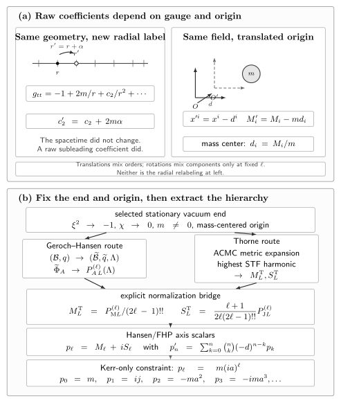
From raw coefficients to stationary multipoles. In the upper panel, the exact redefinition $r'=r+\alpha$ changes subleading coefficients without changing the spacetime, while the translation convention $x'^i=x^i-d^i$ gives $M'_i=M_i-md_i$ and selects $d_i=M_i/m$ in a center-of-mass frame. In the lower panel, a normalized stationary vacuum end can be processed through conformal completion or through an ACMC metric expansion; for nonzero mass, the two routes agree after the displayed Geroch–Hansen-to-Thorne normalization factors are applied. The diagram is schematic and does not assert horizon regularity or a material-source interpretation.

The Geroch–Hansen construction

Let $\xi$ be a stationary Killing field normalized at the selected end by $\xi^2\to-1$. In a neighborhood where it is timelike, define

$$f=-\xi^a\xi_a>0, \qquad q_{ab}=f g_{ab}+\xi_a\xi_b.$$

The second tensor descends to a positive metric on the three-manifold $\mathcal B$ of Killing trajectories. Use the full twist convention of the preceding Ernst page, $d\chi=\varpi$, and fix its additive gauge by $\chi\to0$ at the chosen end.

The asymptotically flat end is compactified by adjoining one regular point $\Lambda$ to $\mathcal B$. A conformal factor $\Omega$ is chosen so that

$$\widetilde q_{ab}=\Omega^2 q_{ab}$$

extends smoothly to $\Lambda$ and satisfies

$$\left.\Omega\right|_\Lambda=0, \qquad \left.\widetilde D_a\Omega\right|_\Lambda=0, \qquad \left.\widetilde D_a\widetilde D_b\Omega\right|_\Lambda =2\left.\widetilde q_{ab}\right|_\Lambda.$$

Here $\widetilde D$ and $\widetilde R_{ab}$ are the derivative and Ricci tensor of $\widetilde q$. The point $\Lambda$ belongs to the compactified orbit space; it should not be confused without qualification with Penrose’s spacetime point $i^0$.

For the site’s sign of $\chi$, the two Hansen potentials are

$$\Phi_{\mathrm M}=\frac{1-f^2-\chi^2}{4f}, \qquad \Phi_{\mathrm J}=-\frac{\chi}{2f}, \qquad \widetilde\Phi_A=\Omega^{-1/2}\Phi_A.$$

This sign is testable rather than conventional decoration: if $f=1-2m/r+O(r^{-2})$ and $\chi=-2j\cos\theta/r^2+O(r^{-3})$, then $\Phi_{\mathrm M}=m/r+O(r^{-2})$ and $\Phi_{\mathrm J}=j\cos\theta/r^2+O(r^{-3})$. Thus the lowest moments will be $m$ and $+j$. The completion, potentials, and smoothness conditions are summarized in Mayerson 2023, §2.1, pp. 4–7, Eqs. (4) and (12)–(19).

For either $A=\mathrm M$ or $A=\mathrm J$, define raw symmetric trace-free tensors by

$$P_A^{(0)}=\widetilde\Phi_A, \qquad P^{(1)}_{A\,a}=\widetilde D_aP_A^{(0)},$$

and, for $n\ge1$,

$$\begin{aligned} P^{(n+1)}_{A\,a_1\ldots a_{n+1}} =\operatorname{STF}\!\Bigl[ &\widetilde D_{a_1}P^{(n)}_{A\,a_2\ldots a_{n+1}}\\ &-\frac{n(2n-1)}2\, \widetilde R_{a_1a_2} P^{(n-1)}_{A\,a_3\ldots a_{n+1}} \Bigr]. \end{aligned}$$

The Ricci term is essential: under an allowed change of conformal factor, it cancels the unwanted dependence on higher derivatives of the rescaling and leaves precisely the expected translation freedom. Evaluated at $\Lambda$, the recursive tensors are the original Geroch–Hansen mass and current moments. Gürsel’s conversion to Thorne’s ACMC tensor normalization is

$$M^{\mathrm T}_{a_1\ldots a_\ell} =\frac{P^{(\ell)}_{\mathrm M\,a_1\ldots a_\ell}(\Lambda)}{(2\ell-1)!!},$$ $$S^{\mathrm T}_{a_1\ldots a_\ell} =\frac{\ell+1}{2\ell(2\ell-1)!!} P^{(\ell)}_{\mathrm J\,a_1\ldots a_\ell}(\Lambda), \qquad \ell\ge1,$$

with $(-1)!!=1$. These factors matter: Geroch–Hansen tensors, Thorne-normalized tensors, and axisymmetric scalar moments are related, but they are not interchangeable names for the same components. The recursion and conversion are given together in Mayerson 2023, §2.1, p. 6, Eqs. (13)–(16). The exact-family formulas below use the conventional Hansen/Fodor–Hoenselaers–Perjés (FHP) axis scalars; every ACMC tensor in the next section carries a superscript $\mathrm T$.

This construction is coordinate independent after the asymptotic end, Killing normalization, twist gauge, and conformal completion are specified, but it remains origin covariant. Residual conformal freedom contains asymptotic translations. Mass-centering removes that freedom when $m\ne0$; without that extra choice, a statement such as “the quadrupole is invariant” is incomplete.

Reading moments in ACMC coordinates

Thorne’s operational route uses asymptotically Cartesian, mass-centered coordinates $x^i$, with $r=(\delta_{ij}x^ix^j)^{1/2}$ and $n^i=x^i/r$. Choose $t$ so that $\partial_t$ approaches the selected future-directed stationary generator, and orient the asymptotic Cartesian triad by $\epsilon_{123}=+1$, consistently with the orientation on the preceding Ernst page. These choices fix the sign of the current-moment term. If $A_\ell=a_1\ldots a_\ell$ is a multi-index, the relevant highest spherical harmonic at each radial order has the form

$$\begin{aligned} g_{tt}={}&-1+\frac{2m}{r}+\frac{\mathcal A^{(tt)}_0}{r^2}\\ &+\sum_{\ell=2}^{\infty}\frac1{r^{\ell+1}} \left[ \frac{2(2\ell-1)!!}{\ell!} M^{\mathrm T}_{A_\ell}n^{A_\ell} +\mathcal A^{(tt)}_{\ell-1} \right], \end{aligned}$$ $$\begin{aligned} g_{tj}=\sum_{\ell=1}^{\infty}\frac1{r^{\ell+1}} \Biggl[ &-\frac{4\ell(2\ell-1)!!}{(\ell+1)!} \epsilon_{jka_\ell}S^{\mathrm T}_{kA_{\ell-1}}n^{A_\ell}\\ &+\mathcal A^{(tj)}_{\ell-1} \Biggr]. \end{aligned}$$

Each $\mathcal A_{\ell-1}$ may contain harmonics only through degree $\ell-1$. The physical moment is the coefficient of the highest allowed harmonic at that radial order. Mass-centering is what excludes an $\ell=1$ harmonic from the $r^{-2}$ part of $g_{tt}$. A coordinate system that permits higher harmonics at a given order is not ACMC, so its coefficients cannot be read with these formulas.

The angular restrictions and read-off rule are detailed in Mayerson 2023, §2.2, pp. 7–8, Eqs. (20)–(21) and in Thorne 1980, §§XI.A–XI.C, pp. 333–336. For stationary asymptotically flat vacuum fields of nonzero mass, Gürsel proved the equivalence of these ACMC tensors and the Geroch–Hansen tensors with exactly the normalization conversion displayed above; see Gürsel 1983, pp. 737–754.

In practice, a safe extraction therefore follows five steps:

1. Choose one asymptotically flat end and normalize $\xi$ and $\chi$ there.
2. Declare whether the calculation uses conformal completion, ACMC coordinates, or a proven equivalent axis algorithm.
3. Fix the origin, normally by setting the mass dipole to zero when $m\ne0$.
4. State the tensor and scalar normalization before quoting numbers.
5. Check dimensions, parity, a spherical limit, and at least one genuinely non-Kerr family.

Axisymmetry, translations, and reflection

Axisymmetry is not needed for the tensor definition above. It merely reduces each STF tensor to one number. Let $z^a$ be the unit vector along the oriented symmetry axis at $\Lambda$. The standard Hansen/FHP scalar convention is

$$\begin{aligned} p_\ell=M_\ell+iS_\ell =\frac1{\ell!}\Bigl[ P^{(\ell)}_{\mathrm M\,a_1\ldots a_\ell} +iP^{(\ell)}_{\mathrm J\,a_1\ldots a_\ell} \Bigr]_{\Lambda} z^{a_1}\cdots z^{a_\ell}. \end{aligned}$$

If one instead writes the ACMC tensors as $M^{\mathrm T}_{A_\ell}=M^{\mathrm T}_\ell z_{\langle A_\ell\rangle}$ and $S^{\mathrm T}_{A_\ell}=S^{\mathrm T}_\ell z_{\langle A_\ell\rangle}$, the conversion above gives

$$M^{\mathrm T}_\ell=M_\ell, \qquad S^{\mathrm T}_\ell=\frac{\ell+1}{2\ell}S_\ell \quad(\ell\ge1).$$

Thus the familiar complex Kerr sequence below is a Hansen/FHP scalar statement. An ACMC current coefficient must be converted before it is inserted into that sequence.

For a translation along the axis with $z'=z-d$, this convention gives the binomial law

$$p'_n=\sum_{k=0}^{n}\binom nk(-d)^{n-k}p_k.$$

In particular, $p'_1=p_1-dp_0$. If $p_0=m>0$ and $p_1=D+iJ$, the real choice $d=D/m$ removes the mass dipole $D$ but leaves the current dipole $J$. The first two transformed orders provide an immediate check that translations mix orders while rotations do not.

Under full spatial parity, mass and current tensors of rank $\ell$ carry factors $(-1)^\ell$ and $(-1)^{\ell+1}$, respectively. Equatorial reflection symmetry therefore forces

$$M_{2k+1}=0, \qquad S_{2k}=0.$$

This statement is separate from reversing the physical spin at a fixed oriented axis. Spin reversal changes the sign of every Kerr current moment but leaves every Kerr mass moment fixed. For example, $S_3$ is even under full parity yet changes sign when the physical spin is reversed. The reflection rule is stated in Fodor, Costa Filho, and Hartmann 2021, p. 064012-2, and their axis-scalar and translation formulas appear in Fodor, Costa Filho, and Hartmann 2021, §III.D, p. 064012-6, Eqs. (42)–(46).

Ernst-axis extraction is nonlinear

For a stationary axisymmetric vacuum field, introduce the Ernst-derived potential

$$\Xi=\frac{1-\mathcal E}{1+\mathcal E}.$$

In a mass-centered Weyl coordinate $z$ on the north axis, set $\bar z=1/z$ and compactify the potential as

$$\widetilde\Xi(\bar z) =\bar z^{-1}\Xi(\bar z^{-1}) =\sum_{n=0}^{\infty}m_n\bar z^n.$$

The coefficients $m_n$ are useful input data, but the field equations and the curvature term in the Geroch–Hansen recursion make the final map nonlinear. In vacuum,

$$p_0=m_0, \qquad p_1=m_1, \qquad p_2=m_2, \qquad p_3=m_3,$$

whereas

$$p_4=m_4-\frac17\overline{m}_0\left(m_2m_0-m_1^2\right).$$

Asymptotic flatness with the standard mass normalization gives $m_0=\overline m_0=m\in\mathbb R$. Thus even a correctly normalized, mass-centered axis-potential coefficient need not equal the relativistic moment at the same order. The corrected algorithm and this first vacuum nonlinear term appear in Fodor, Costa Filho, and Hartmann 2021, §IV.C, p. 064012-11, especially Eqs. (84) and (86)–(90). Electrovacuum requires a coupled gravitational-electromagnetic extension; applying the vacuum one-potential rule there is not valid.

Kerr: a complete normalization lock

The Kerr metric page defines $j=ma$. In the twist convention used here, its Ernst potential is

$$\mathcal E_{\mathrm{Kerr}} =1-\frac{2m}{r-ia\cos\theta}.$$

Therefore

$$\Xi=\frac{m}{r-m-ia\cos\theta}.$$

The associated Weyl coordinate is $z=(r-m)\cos\theta$. On the north axis,

$$\Xi=\frac{m}{z-ia}, \qquad \widetilde\Xi=\frac{m}{1-ia\bar z} =\sum_{n=0}^{\infty}m(ia)^n\bar z^n.$$

For this special geometric sequence, every nonlinear correction cancels, and the complete hierarchy is

$$\boxed{p_\ell=M_\ell+iS_\ell=m(ia)^\ell.}$$

Hence

$$M_0=m, \qquad S_1=ma=j, \qquad M_2=-ma^2, \qquad S_3=-ma^3.$$

The same Hansen/FHP convention is used in the Kerr–Newman statement of Fodor, Costa Filho, and Hartmann 2021, p. 064012-13; setting the charge to zero gives the sequence above. Three independent checks now agree: $a\to0$ leaves only the Schwarzschild monopole, $a\to-a$ flips all current moments at fixed axis orientation, and every order has dimension $L^{\ell+1}$. The boxed identity is a property of Kerr, not a universal relation for rotating bodies.

Zipoy–Voorhees: why an axis coefficient is not a moment

The static Zipoy–Voorhees family supplies an inequivalent test. On the north symmetry axis, write its Ernst potential as

$$\mathcal E_{\mathrm{ZV}} =\left(\frac{z-\sigma}{z+\sigma}\right)^\delta.$$

Direct expansion gives

$$\begin{aligned} \widetilde\Xi={}&\delta\sigma +\frac{\delta(1-\delta^2)\sigma^3}{3}\bar z^2\\ &+\frac{\delta(1-\delta^2)(3-2\delta^2)\sigma^5}{15}\bar z^4 +O(\bar z^6). \end{aligned}$$

Reflection symmetry and staticity make all odd mass moments and all current moments vanish. The first moments are

$$M_0=\delta\sigma, \qquad M_2=\frac{\delta(1-\delta^2)\sigma^3}{3},$$

in agreement with the exact family data in Mejía, Manko, and Ruiz 2019, §II, pp. 3–5, Eqs. (3)–(6). But at order four the nonlinear correction matters:

$$\begin{aligned} M_4 &=m_4-\frac17m_0^2m_2\\ &=\frac{\delta(1-\delta^2)(21-19\delta^2)\sigma^5}{105}. \end{aligned}$$

For generic $\delta$, this is not the coefficient $m_4$ displayed in $\widetilde\Xi$. At $\delta=1$ the solution reduces to Schwarzschild with mass $\sigma$ and every higher moment vanishes; at $\delta=0$ it is flat. The family therefore checks the spherical limit, the reflection rule, the quadrupole sign, and—most importantly—the distinction between series data and invariantly normalized moments.

What the hierarchy does and does not determine

A full convergent hierarchy carries much more information than a few fitted coefficients. Under the stationary vacuum analyticity hypotheses, two solutions with the same complete moments—after matching the end normalization and origin—are locally isometric near that infinity; see Beig and Simon 1981, pp. 333 and 340. This is a local asymptotic statement. It does not by itself prove that the interior contains a regular horizon, exclude a material surface or singularity, determine global topology, establish stability, or identify a second disconnected asymptotic end.

Nor can a finite list identify a generic exact spacetime. Agreement with Kerr through $M_2$, for example, leaves infinitely many higher moments and all global conditions unchecked. A meaningful “Kerr multipole test” must declare the frame, normalization, inferred orders, uncertainties, and model class rather than treating $M_0$ and $S_1$ alone as no-hair evidence.

Common pitfalls

Calling every coefficient a moment. A coefficient becomes a moment only after the asymptotic gauge and normalization have been controlled, or after a theorem maps the chosen data to the Geroch–Hansen hierarchy.

Calling the hierarchy origin invariant. The construction is coordinate independent but translations act covariantly on the hierarchy. State the origin convention; for nonzero mass, a vanishing mass dipole is the standard choice.

Using parity to explain spin reversal. Full spatial parity and the physical comparison $J\to-J$ are different operations. Current moments have parity $(-1)^{\ell+1}$, while every Kerr current moment is odd under physical spin reversal.

Using the Kerr relation as a definition. $p_\ell=m(ia)^\ell$ is a stringent family identity. A generic rotating star or non-Kerr vacuum exterior has independent higher moments.

Exercises

1. Radial-gauge contamination

Starting from

$$g_{tt}=-1+\frac{2m}{r}+\frac{c_2}{r^2}+\frac{c_3}{r^3}+O(r^{-4}),$$

derive $c'_2$ and $c'_3$ under the exact change $r'=r+\alpha$. Why would the result for $c'_3$ be underdetermined if the change were stated only as $r'=r+\alpha+O(r^{-1})$?

Solution

Because $r=r'-\alpha$,

$$r^{-1}=r'^{-1}+\alpha r'^{-2}+\alpha^2r'^{-3}+O(r'^{-4}),$$ $$r^{-2}=r'^{-2}+2\alpha r'^{-3}+O(r'^{-4}), \qquad r^{-3}=r'^{-3}+O(r'^{-4}).$$

Collecting equal powers gives

$$c'_2=c_2+2m\alpha, \qquad c'_3=c_3+2\alpha c_2+2m\alpha^2.$$

If $r'=r+\alpha+\beta/r+\cdots$, the unknown $\beta$ contributes to $r^{-1}$ at order $r'^{-3}$. The $\alpha^2$ term alone is therefore not determined by the abbreviated transformation.

2. Centering a complex axis hierarchy

Let $p_0=m>0$, $p_1=D+iJ$, and $p_2=Q+iC$. Under $z'=z-d$, find the real $d$ that removes the mass dipole. What are $p'_1$ and $p'_2$?

Solution

The binomial translation law gives

$$p'_1=p_1-dp_0=D-md+iJ.$$

Choose $d=D/m$. Then $p'_1=iJ$: centering removes the mass dipole, not the angular momentum. At the next order,

$$\begin{aligned} p'_2 &=p_2-2dp_1+d^2p_0\\ &=Q-\frac{D^2}{m} +i\left(C-\frac{2DJ}{m}\right). \end{aligned}$$

The result displays explicitly how a translation mixes lower moments into higher ones.

3. Reflection symmetry versus spin reversal

List the moments through $\ell=5$ allowed by equatorial reflection symmetry. Then apply physical spin reversal to the Kerr sequence and explain why this is not the same rule as full spatial parity.

Solution

Equatorial reflection permits

$$M_0,\ S_1,\ M_2,\ S_3,\ M_4,\ S_5$$

and sets $M_1,S_2,M_3,S_4,M_5$ to zero. For Kerr, $p_\ell=m(ia)^\ell$. Sending $a\to-a$ leaves every even-$\ell$ mass moment unchanged and flips every odd-$\ell$ current moment. Full spatial parity instead assigns a current rank-$\ell$ tensor the factor $(-1)^{\ell+1}$; thus $S_3$ is parity even although it flips under physical spin reversal. The two operations answer different questions.

4. The first nonlinear axis correction

For Zipoy–Voorhees, use

$$m_0=\delta\sigma, \quad m_2=\frac{\delta(1-\delta^2)\sigma^3}{3}, \quad m_4=\frac{\delta(1-\delta^2)(3-2\delta^2)\sigma^5}{15}$$

and $p_4=m_4-m_0^2m_2/7$ to derive $M_4$. Check $\delta=1$ and explain what the calculation proves about $m_4$.

Solution

Substitution gives

$$\begin{aligned} M_4 &=\delta(1-\delta^2)\sigma^5 \left[\frac{3-2\delta^2}{15}-\frac{\delta^2}{21}\right]\\ &=\frac{\delta(1-\delta^2)(21-19\delta^2)\sigma^5}{105}. \end{aligned}$$

At $\delta=1$, the factor $1-\delta^2$ makes $M_4=0$, as Schwarzschild requires. For generic $\delta$, the subtraction is nonzero, so the fourth compactified axis coefficient $m_4$ is not the fourth relativistic moment.

The next page uses the same stationary quotient to distinguish ergoregions, Killing horizons, and axis segments. That global analysis is deliberately separate: asymptotic moments alone do not certify a regular horizon.

References

• Beig, Robert, and Walter Simon. “On the Multipole Expansion for Stationary Space-Times.” Proceedings of the Royal Society of London A 376, no. 1765 (1981): 333–341. DOI: 10.1098/rspa.1981.0095.
• Fodor, Gyula, Etevaldo dos Santos Costa Filho, and Betti Hartmann. “Calculation of Multipole Moments of Axistationary Electrovacuum Spacetimes.” Physical Review D 104, no. 6 (2021): 064012. DOI: 10.1103/PhysRevD.104.064012.
• Geroch, Robert. “Multipole Moments. II. Curved Space.” Journal of Mathematical Physics 11, no. 8 (1970): 2580–2588. DOI: 10.1063/1.1665427.
• Gürsel, Yekta. “Multipole Moments for Stationary Systems: The Equivalence of the Geroch–Hansen Formulation and the Thorne Formulation.” General Relativity and Gravitation 15, no. 8 (1983): 737–754. DOI: 10.1007/BF01031881.
• Hansen, R. O. “Multipole Moments of Stationary Space-Times.” Journal of Mathematical Physics 15, no. 1 (1974): 46–52. DOI: 10.1063/1.1666501.
• Mayerson, Daniel R. “Gravitational Multipoles in General Stationary Spacetimes.” SciPost Physics 15, no. 4 (2023): 154. DOI: 10.21468/SciPostPhys.15.4.154.
• Mejía, I. M., V. S. Manko, and E. Ruiz. “On the Simplest Static and Stationary Vacuum Quadrupolar Metrics.” Physical Review D 100, no. 12 (2019): 124021. DOI: 10.1103/PhysRevD.100.124021.
• Thorne, Kip S. “Multipole Expansions of Gravitational Radiation.” Reviews of Modern Physics 52, no. 2 (1980): 299–339. DOI: 10.1103/RevModPhys.52.299.