Schwarzschild Coordinate Atlas

The Schwarzschild geometry is one spacetime with many useful coordinate systems. No single familiar chart simultaneously makes the exterior static symmetry diagonal, follows freely falling observers, crosses both horizon branches, and displays the entire analytic extension. This page builds a working atlas: every transformation comes with its metric, domain, horizon branch, Killing field, and one invariant check. For the field-equation calculation that produces the geometry, begin with Deriving the Schwarzschild Metric.

Required background. The Einstein Equation supplies the vacuum solution being re-charted.

Helpful background. The Riemann Curvature Tensor supports coordinate-independent checks; Exact Solutions of Einstein’s Equations supplies the coordinate-domain discipline; Causality and Global Structure supplies the language of horizons and extensions; Affine and Variational Geodesics explains the infalling congruences behind the free-fall charts.

Areal radius and the horizon-crossing test

Let

$$r_s=2GM\gt0, \qquad f(r)=1-\frac{r_s}{r}.$$

The coordinate $r$ is the areal radius: every symmetry sphere has area $4\pi r^2$. It is therefore a geometrically defined scalar, not merely the name of one coordinate. In the right exterior, Schwarzschild coordinates give

$$ds^2=-f\,dt^2+f^{-1}dr^2+r^2d\Omega_2^2, \qquad r\gt r_s,$$

and the future-directed Killing field normalized at that infinity is $\xi=\partial_t$. The metric is stationary because its components are independent of $t$, and it is manifestly static because it is diagonal and $\xi$ is orthogonal to the $t=\text{constant}$ slices. These are stronger statements than “the spacetime has a static exterior.”

To say that a chart crosses a selected horizon branch, check all three facts:

1. its domain contains the horizon and points on both sides;
2. the metric and inverse metric have finite smooth components there; and
3. the metric remains nondegenerate there.

A finite determinant by itself is not enough. The singular Schwarzschild radial block already has determinant $-1$, because the zero of $g_{tt}$ and the pole of $g_{rr}$ cancel in that product. Its components and inverse do not remain smooth at $r=r_s$, and the exterior chart does not contain points across that boundary.

There are two logically distinct steps in a horizon extension. On an overlap such as $r\gt r_s$, a formula like $v=t+r_*$ is an ordinary coordinate change between points already in both charts. That change of variables is singular at $r=r_s$. What permits a local extension is instead that the metric rewritten in $(v,r)$ has a smooth, nondegenerate continuation there. One glues a new chart carrying that continuation to the exterior through their regular overlap; the new chart’s domain includes points on and across the horizon. One should not imagine applying a singular coordinate transformation to a horizon point that was already present in the exterior Schwarzschild chart.

The areal radius supplies a coordinate-independent local check:

$$\nabla_a r\,\nabla^a r=f(r).$$

The radius gradient is spacelike in either exterior, null at $r=r_s$, and timelike in either interior. Away from the bifurcation sphere, where $dr\ne0$, this shows that $r=r_s$ is a null level hypersurface. At the bifurcation sphere $dr=0$ and the two branches meet. The scalar by itself neither distinguishes the future branch from the past branch nor proves the global event-horizon property.

Here is the atlas at a glance. Throughout this page, I is the right exterior, II the black-hole interior, III the left exterior, and IV the white-hole interior. Roman-numeral conventions are not universal: Reall 2013, §§12.5–12.6, pp. 141–148, Open PDF uses III for the white-hole interior and IV for the left exterior. “Coverage from I” means that the chart is normalized in the selected right exterior; the exact Kruskal signs appear below.

Chart	Coverage from Region I	Horizon crossing	Time or slicing structure
Schwarzschild $(t,r)$	I	neither branch	Killing time; manifestly static
Tortoise $(t,r_*)$	I	neither; the horizon lies at $r_*\to-\infty$	Killing time; radial null rays have slope $\pm1$
Advanced Eddington–Finkelstein $(v,r)$	I and II	future branch	time independent; $\partial_v=\xi$; time–radius cross term
Retarded Eddington–Finkelstein $(u,r)$	I and IV	past branch	time independent; $\partial_u=\xi$; time–radius cross term
Ingoing Painlevé–Gullstrand $(T_+,r)$	I and II	future branch	time independent; $\partial_{T_+}=\xi$; flat spatial slices
Outgoing Painlevé–Gullstrand $(T_-,r)$	I and IV	past branch	time independent; $\partial_{T_-}=\xi$; flat spatial slices
Ingoing Lemaître $(\tau,R)$	I and II	future branch	comoving free-fall time; not manifestly stationary
Outgoing Lemaître $(\tau_-,R_-)$	I and IV	past branch	comoving outgoing free fall; not manifestly stationary
Isotropic $(t,\rho)$	I for $\rho\gt r_s/4$; separate III branch for $0\lt\rho\lt r_s/4$	neither branch	conformally flat spatial metric; future static time is $t$ in I and $-t$ in III
Kruskal–Szekeres $(U,V)$	I, II, III, and IV	both branches and their intersection	Killing symmetry is a boost, not a coordinate-time translation

The static metric and its domain are reviewed in Reall 2013, §12.1, pp. 131–133, Open PDF.

Tortoise and Eddington–Finkelstein coordinates

For a radial null curve, $d\Omega_2=0$ and $ds^2=0$ imply

$$\frac{dt}{dr}=\pm f^{-1}.$$

This motivates the tortoise coordinate

$$r_*=r+r_s\ln\left|\frac{r}{r_s}-1\right|, \qquad \frac{dr_*}{dr}=f^{-1}.$$

In Region I, approaching the horizon radius sends $r_*\to-\infty$; this radial limit alone does not select a horizon branch. Define $u=t-r_*$ and $v=t+r_*$. Outgoing radial null rays have constant $u$, whereas ingoing rays have constant $v$. Keeping $v$ finite while $r_*\to-\infty$ selects the future branch $U=0,V\gt0$; keeping $u$ finite selects the past branch $V=0,U\lt0$. The same coordinates put the radial metric in the simple double-null form

$$ds_{\mathrm{rad}}^2=-f\,du\,dv.$$

The tortoise coordinate is excellent for wave propagation, but it has not crossed the horizon: it has moved the horizon to an infinite coordinate location.

Now keep the advanced coordinate $v$ and return from $r_*$ to the areal radius $r$. Because $dt=dv-f^{-1}dr$,

$$ds^2=-f\,dv^2+2\,dv\,dr+r^2d\Omega_2^2.$$

The radial metric and inverse in $(v,r)$ are

$$g_{ab}= \begin{pmatrix} -f&1\\ 1&0 \end{pmatrix}, \qquad g^{ab}= \begin{pmatrix} 0&1\\ 1&f \end{pmatrix}, \qquad \det g_{ab}=-1.$$

Every entry is smooth at $r=r_s$. With $v\in\mathbb R$ and $r\gt0$, this advanced chart covers the right exterior I, the future horizon $U=0,V\gt0$, and black-hole Region II. It does not include the bifurcation sphere or the past horizon.

The retarded coordinate $u$ instead gives

$$ds^2=-f\,du^2-2\,du\,dr+r^2d\Omega_2^2.$$

With $u\in\mathbb R$ and $r\gt0$, it covers I, the past horizon $V=0,U\lt0$, and white-hole Region IV. Both metrics are time independent and adapted to the Killing field: $\partial_v=\partial_u=\xi$ on their respective overlaps with the static exterior. There $\xi$ is timelike, but it becomes null at the selected horizon and spacelike in the adjacent interior. Thus the chart remains Killing-adapted, but $\xi$ represents timelike stationary observers only in I; the time–radius cross term also hides the exterior’s orthogonal static slicing. The exact transformations and the corresponding horizon branches appear in Reall 2013, §§12.5–12.6, pp. 141–148, Open PDF.

Painlevé–Gullstrand and Lemaître free-fall charts

It is helpful to abbreviate $q(r)=\sqrt{r_s/r}$. Choose the ingoing Painlevé–Gullstrand time by

$$dT_+=dt+\frac{q}{f}\,dr.$$

On either side of the horizon, where the static coordinate $t$ is separately defined, integration gives

$$T_+=t+2\sqrt{r_s r} +r_s\ln\left| \frac{\sqrt r-\sqrt{r_s}}{\sqrt r+\sqrt{r_s}} \right|.$$

Substitution produces

$$\begin{aligned} ds^2 &=-f\,dT_+^2+2q\,dT_+\,dr+dr^2+r^2d\Omega_2^2\\ &=-dT_+^2+\left(dr+q\,dT_+\right)^2 +r^2d\Omega_2^2. \end{aligned}$$

The radial determinant is again $-1$. Setting $dT_+=0$ leaves $dr^2+r^2d\Omega_2^2$, so every $T_+=\text{constant}$ slice is intrinsically Euclidean on the punctured domain $r\gt0$. This does not make the spacetime flat: the shift and the extrinsic curvature of the slices still carry gravitational information. The future-directed unit normal on the exterior overlap is

$$n_+=\partial_{T_+}-q\,\partial_r.$$

The coordinates obey $T_+\in\mathbb R$, $r\gt0$ and cover I plus II; the metric is time independent with $\partial_{T_+}=\xi$.

The outgoing, past-penetrating partner is not merely a verbal sign choice. It is defined by

$$dT_-=dt-\frac{q}{f}\,dr,$$

so, on either side of the horizon within a separate Schwarzschild-coordinate domain,

$$T_-=t-2\sqrt{r_s r} -r_s\ln\left| \frac{\sqrt r-\sqrt{r_s}}{\sqrt r+\sqrt{r_s}} \right|.$$

Its metric is

$$ds^2=-dT_-^2+\left(dr-q\,dT_-\right)^2+r^2d\Omega_2^2, \qquad n_-=\partial_{T_-}+q\,\partial_r.$$

Both completed-square metrics have unit lapse, so the slice-normal acceleration $D_a\ln N$ vanishes and $n_\pm$ are geodesic. Direct substitution also gives the beginner-useful checks

$$n_\pm^2=-1, \qquad -\xi\!\cdot n_\pm=1, \qquad n_\pm(r)=\mp\sqrt{\frac{r_s}{r}}.$$

Thus $n_+$ is the congruence dropped from rest at infinity: its Killing energy per unit mass is one and its areal radius decreases. The $n_-$ congruence is its time reverse; it moves outward and approaches zero speed at infinity. Here $T_-\in\mathbb R$, $r\gt0$, and the chart covers I plus IV across the past horizon. It remains time independent, with $\partial_{T_-}=\xi$. In both PG charts, $\xi$ is timelike only in I, null on the selected horizon, and spacelike in the interior. Martel and Poisson derive this family from radial geodesic energy in Martel and Poisson 2001, §§II–III, arXiv v4 PDF pp. 2–4, Open PDF.

Lemaître coordinates make the same ingoing congruence comoving. We reserve the unsubscripted pair $(\tau,R)$ for this ingoing branch and define

$$d\tau=dt+\frac{\sqrt{r_s/r}}{f}\,dr, \qquad dR=dt+\frac{\sqrt{r/r_s}}{f}\,dr.$$

Subtracting gives

$$dR-d\tau=\sqrt{\frac{r}{r_s}}\,dr, \qquad r=\left[\frac32\sqrt{r_s}\,(R-\tau)\right]^{2/3}.$$

The metric becomes

$$ds^2=-d\tau^2+\frac{r_s}{r}\,dR^2+r^2d\Omega_2^2, \qquad R-\tau\gt0, \qquad \tau,R\in\mathbb R.$$

Its radial block, inverse, and determinant are

$$g^{\mathrm{rad}}_{ab}=\operatorname{diag}\!\left(-1,\frac{r_s}{r}\right), \qquad g_{\mathrm{rad}}^{ab}=\operatorname{diag}\!\left(-1,\frac{r}{r_s}\right), \qquad \det g^{\mathrm{rad}}_{ab}=-\frac{r_s}{r}.$$

At $r=r_s$ all entries are finite and the determinant is $-1$, so this chart passes the full local horizon-crossing test rather than only a determinant test.

Worldlines $R=\text{constant}$ have proper time $\tau$ and fall toward smaller $r$. The future horizon is the regular line $R-\tau=2r_s/3$, while the curvature-singular boundary is $R=\tau$. The metric components depend on $R-\tau$, so $\partial_\tau$ is not Killing. Instead,

$$\xi=\partial_\tau+\partial_R, \qquad \xi^2=-1+\frac{r_s}{r}=-f.$$

Thus the underlying exterior is still static even though the chart hides the symmetry. For completeness, the outgoing chart is defined explicitly by

$$d\tau_-=dt-\frac{q}{f}\,dr, \qquad dR_-=dt-\frac{q^{-1}}{f}\,dr.$$

Now

$$d\tau_--dR_-=q^{-1}dr, \qquad r=\left[\frac32\sqrt{r_s}\,(\tau_--R_-)\right]^{2/3},$$

and

$$ds^2=-d\tau_-^2+\frac{r_s}{r}\,dR_-^2+r^2d\Omega_2^2, \qquad \tau_--R_-\gt0, \qquad \tau_-,R_-\in\mathbb R.$$

The outgoing radial block has the same inverse and determinant, and is equally regular at its selected horizon.

Worldlines $R_-=\text{constant}$ move toward larger $r$ as $\tau_-$ increases. The past horizon is the regular line $\tau_--R_-=2r_s/3$, the singular boundary is $\tau_-=R_-$, and $\xi=\partial_{\tau_-}+\partial_{R_-}$. This chart covers I plus IV. Gourgoulhon derives the ingoing Lemaître and Painlevé–Gullstrand constructions, including their Killing and free-fall interpretations, in Gourgoulhon 2026, §§14.2.6–14.2.7, pp. 553–556, official author PDF. The outgoing formulas above are their explicit time reverses.

Isotropic radius and the two exterior ends

To make a static spatial metric conformally flat, write

$$f^{-1}dr^2+r^2d\Omega_2^2 =\psi^4\left(d\rho^2+\rho^2d\Omega_2^2\right).$$

Matching the angular and radial parts gives $r=\psi^2\rho$. The radial equation has opposite monotonic branches:

$$\frac{d\rho}{\rho} =\begin{cases} +\dfrac{dr}{r\sqrt f},&\rho\gt r_s/4,\\[4pt] -\dfrac{dr}{r\sqrt f},&0\lt\rho\lt r_s/4. \end{cases}$$

Integrating the first branch and fixing $\rho/r\to1$ at the right infinity gives a relation that contains both branches:

$$r=\rho\left(1+\frac{r_s}{4\rho}\right)^2, \qquad \psi=1+\frac{r_s}{4\rho}.$$

For any fixed $r\gt r_s$, its two inverse values are

$$\rho_\pm(r)=\frac12\left( r-\frac{r_s}{2}\pm\sqrt{r(r-r_s)} \right),$$

with $\rho_+\gt r_s/4$ and $0\lt\rho_-\lt r_s/4$.

The complete four-metric is

$$ds^2 =-\left(\frac{1-r_s/(4\rho)}{1+r_s/(4\rho)}\right)^2dt^2 +\left(1+\frac{r_s}{4\rho}\right)^4 \left(d\rho^2+\rho^2d\Omega_2^2\right).$$

Two elementary checks reveal its domain:

$$\frac{dr}{d\rho} =\frac{(4\rho-r_s)(4\rho+r_s)}{16\rho^2}, \qquad r\left(\frac{r_s^2}{16\rho}\right)=r(\rho).$$

The branch $\rho\gt r_s/4$ represents Region I. The Jacobian vanishes at $\rho=r_s/4$, where $r=r_s$ and the four-metric written above degenerates, so this chart does not cross the horizon. At finite Schwarzschild $t$, approaching this locus from either branch tends to the bifurcation two-sphere $B$: all finite values of $t$ collapse to the same limiting sphere, so the displayed map is not injective there. Neither open isotropic branch includes $B$; other horizon points require a correlated limit with $|t|\to\infty$. The inversion-related branch $0\lt\rho\lt r_s/4$ can represent the second exterior Region III in the eternal extension: as $\rho\to0$, its areal radius again tends to infinity. The two values of $\rho$ with the same $r$ are different spacetime points in that two-ended construction, not duplicate coordinate labels for one point. The same global Killing parameter $t$ makes $\partial_t$ future-directed in I but past-directed in III. A future-directed static time at the left infinity is therefore $t_L=-t$. See Gourgoulhon 2026, §9.5.3, pp. 324–326, official author PDF for the exact metric and two-exterior interpretation.

Kruskal coordinates across both horizon branches

In Region I, fix the signs rather than writing an ambiguous $\pm$:

$$U=-e^{-u/(2r_s)}, \qquad V=e^{v/(2r_s)}.$$

Their product removes $t$ and determines the areal radius implicitly:

$$-UV=\left(\frac{r}{r_s}-1\right)e^{r/r_s}.$$

Since $(x-1)e^x$ is strictly increasing for $x=r/r_s\gt0$ and maps that interval to $(-1,\infty)$, the physical radial domain is exactly

$$UV\lt1.$$

The metric is

$$ds^2 =-\frac{4r_s^3}{r}e^{-r/r_s}\,dU\,dV+r^2d\Omega_2^2.$$

With $\mathsf T_K=(U+V)/2$ and $\mathsf X_K=(V-U)/2$, its radial part is

$$ds_{\mathrm{rad}}^2 =\frac{4r_s^3}{r}e^{-r/r_s} \left(-d\mathsf T_K^2+d\mathsf X_K^2\right).$$

It is therefore conformal to the two-dimensional Minkowski metric, and radial null rays run at $45^\circ$. The figure uses these uncompactified Kruskal coordinates; unlike a Penrose diagram, it does not bring infinity to a finite boundary.

At either horizon, $UV=0$ and $r=r_s$, so the coefficient of $-dU\,dV$ tends to $4r_s^2/e$: it is finite and nonzero. Allowing $U$ and $V$ to take both signs gives four connected sectors:

Region	Sign of $U$	Sign of $V$	Interpretation
I	negative	positive	selected right exterior
II	positive	positive	black-hole interior
III	positive	negative	left exterior
IV	negative	negative	white-hole interior

The future horizon has two half-branches, $U=0,V\gt0$ and $V=0,U\gt0$; the past horizon has $V=0,U\lt0$ and $U=0,V\lt0$. All four meet at the bifurcation sphere $B=(0,0)$. The curvature-singular boundary $r=0$ lies at $UV=1$ and is excluded. Choose the global future direction so that future-directed radial causal curves have nondecreasing $U$ and $V$. The normalized Killing field becomes the boost generator

$$\xi=\frac{1}{2r_s} \left(V\partial_V-U\partial_U\right), \qquad \xi^2=-f.$$

Consequently $\xi$ is future-directed timelike in I, past-directed timelike in III, null on the horizons (and zero at $B$), and spacelike in II and IV. A single Killing field cannot agree with the future-directed static clocks at both asymptotic ends.

The figure compares the exact domains. Inspect the shaded sectors, the thick horizon half-branch selected by each one-horizon family, and whether the bifurcation sphere is open or filled.

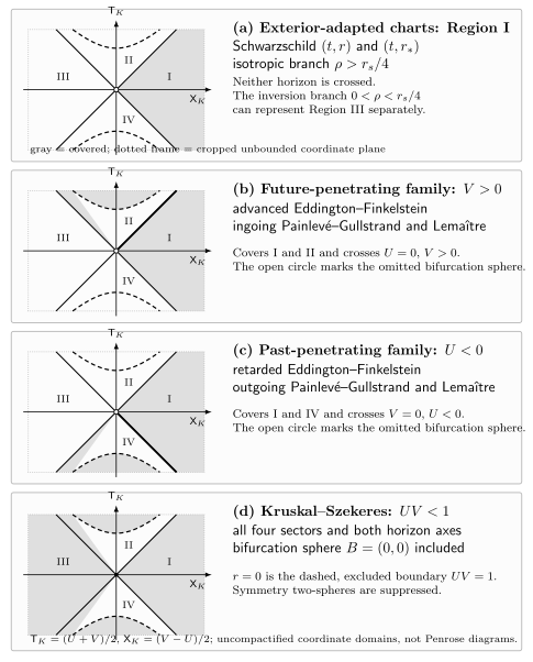
With the Region-I normalization $U=-e^{-u/(2r_s)}$ and $V=e^{v/(2r_s)}$, exterior-adapted charts remain in I; advanced Eddington–Finkelstein and the ingoing Painlevé–Gullstrand and Lemaître charts cover I and II across $U=0,V\gt0$; their retarded or outgoing partners cover I and IV across $V=0,U\lt0$; and Kruskal–Szekeres covers all four sectors and includes $B=(0,0)$. The physical radial domain is $UV\lt1$, with $r=0$ the dashed excluded boundary $UV=1$. These exact coordinate-domain diagrams crop the unbounded exteriors, suppress the symmetry two-spheres, and are uncompactified Kruskal-coordinate plots rather than Penrose compactifications; they carry no proper-distance scale.

The original construction and sector table are in Kruskal 1960, pp. 1743–1745, Tables I–II and Figs. 1–2. For the causal meaning of all four regions, continue to The Maximal Schwarzschild Extension.

Invariant agreement and choosing a chart

Every chart above describes the same vacuum curvature wherever their domains overlap. Because $r$ is the invariant areal radius, the Kretschmann scalar has the same expression in all of them:

$$R_{abcd}R^{abcd} =\frac{48G^2M^2}{r^6} =\frac{12r_s^2}{r^6}.$$

It equals $12/r_s^4$ at the horizon, diverges as $r\to0$, and tends to zero when $M\to0$ at fixed $r\gt0$. This cleanly separates the regular horizon from the true curvature singularity. It also explains why changing coordinates can remove the static pole but cannot remove the centre.

Choose a chart for the structure you need:

• use Schwarzschild time for exterior static observables and conserved Killing energy;
• use $u$, $v$, or $r_*$ for radial characteristics and wave propagation;
• use ingoing Eddington–Finkelstein or Painlevé–Gullstrand coordinates for future-horizon penetration;
• use Lemaître coordinates when the freely falling congruence should be comoving;
• use isotropic coordinates for conformally flat exterior spatial geometry and two-ended initial-slice intuition; and
• use Kruskal coordinates when both horizon branches and the analytic four-region extension matter.

Common pitfalls

Regular at one horizon is not maximal. Advanced Eddington–Finkelstein, ingoing Painlevé–Gullstrand, and ingoing Lemaître coordinates cross the future branch from Region I, but they omit the past branch, Region III, Region IV, and the bifurcation sphere.

Flat slices do not imply flat spacetime. Painlevé–Gullstrand $T_\pm=\text{constant}$ slices have zero intrinsic curvature. Their nonzero extrinsic curvature, and the nonzero four-dimensional Kretschmann scalar, still encode gravity.

The same areal radius is not the same event. Isotropic inversion gives two values of $\rho$ with the same $r$. In the two-ended extension they label different points in different exteriors.

Time-independent components do not make the Killing direction timelike everywhere. Eddington–Finkelstein and Painlevé–Gullstrand metrics are time independent and adapted to the same Killing field, but that field is timelike only in the exterior. Their time–radius cross terms also hide the orthogonal static slicing there. Lemaître coordinates hide even time independence.

Exercises

1. Why the advanced chart crosses the future horizon

Starting from $dt=dv-f^{-1}dr$, derive the advanced Eddington–Finkelstein radial metric, its inverse, and its determinant. Explain why this proves more than the static determinant alone.

Solution

Substitution gives

$$\begin{aligned} -f\,dt^2+f^{-1}dr^2 &=-f\left(dv-f^{-1}dr\right)^2+f^{-1}dr^2\\ &=-f\,dv^2+2\,dv\,dr. \end{aligned}$$

Thus

$$g_{ab}= \begin{pmatrix} -f&1\\ 1&0 \end{pmatrix}, \qquad g^{ab}= \begin{pmatrix} 0&1\\ 1&f \end{pmatrix}, \qquad \det g_{ab}=-1.$$

Both matrices have finite smooth entries at $f=0$, and the domain $v\in\mathbb R$, $r\gt0$ includes $r$ on both sides of $r_s$. By contrast, the static block $\operatorname{diag}(-f,f^{-1})$ also has determinant $-1$, but its metric and inverse contain divergent entries and its exterior domain ends at the horizon. Along future-directed ingoing null rays, $v$ stays finite; in Kruskal signs this regular boundary is $U=0,V\gt0$. That selects the future horizon rather than the past one.

2. What is flat in Painlevé–Gullstrand coordinates?

Integrate the ingoing time transformation, recover the completed-square form of the metric, and determine the intrinsic geometry of a $T_+=\text{constant}$ slice. Then give one invariant reason the spacetime is not flat.

Solution

Set $y=\sqrt{r/r_s}$. Since $dr=2r_s y\,dy$,

$$\int\frac{\sqrt{r_s/r}}{f}\,dr =2r_s\int\frac{y^2}{y^2-1}\,dy =2\sqrt{r_s r} +r_s\ln\left| \frac{\sqrt r-\sqrt{r_s}}{\sqrt r+\sqrt{r_s}} \right|.$$

Using $dt=dT_+-\sqrt{r_s/r}\,f^{-1}dr$ gives

$$ds^2=-dT_+^2+ \left(dr+\sqrt{\frac{r_s}{r}}\,dT_+\right)^2+r^2d\Omega_2^2.$$

At $dT_+=0$, the induced metric is $dl^2=dr^2+r^2d\Omega_2^2$, the Euclidean metric in spherical coordinates on the punctured domain $r\gt0$. The four-dimensional curvature is nevertheless nonzero: $R_{abcd}R^{abcd}=12r_s^2/r^6$.

3. Derive the ingoing Lemaître chart

Starting from the ingoing Painlevé–Gullstrand metric, set $d\tau=dT_+$ and $dR-d\tau=q^{-1}dr$. Derive $r(\tau,R)$, the diagonal metric, its radial determinant and inverse, and the Killing field. Locate the future horizon and the curvature-singular boundary. Why is $\partial_\tau$ comoving but not Killing?

Solution

The coordinate relation immediately gives

$$dr=q(dR-d\tau).$$

The completed-square radial metric therefore becomes

$$-d\tau^2+(dr+q\,d\tau)^2 =-d\tau^2+q^2dR^2.$$

Integrating $dR-d\tau=q^{-1}dr=\sqrt{r/r_s}\,dr$ gives

$$R-\tau=\frac{2r^{3/2}}{3\sqrt{r_s}}, \qquad r=\left[\frac32\sqrt{r_s}\,(R-\tau)\right]^{2/3}.$$

Thus

$$ds^2=-d\tau^2+\frac{r_s}{r}\,dR^2+r^2d\Omega_2^2,$$

and

$$g^{\mathrm{rad}}_{ab}=\operatorname{diag}\!\left(-1,\frac{r_s}{r}\right), \qquad g_{\mathrm{rad}}^{ab}=\operatorname{diag}\!\left(-1,\frac{r}{r_s}\right), \qquad \det g^{\mathrm{rad}}_{ab}=-\frac{r_s}{r}.$$

At $r=r_s$, the radial block and its inverse both reduce to $\operatorname{diag}(-1,1)$, so smoothness and nondegeneracy are explicit. Along $R=\text{constant}$, differentiating the radius relation instead gives $dr/d\tau=-q$, recovering the same infalling congruence as $n_+$ in the Painlevé–Gullstrand chart.

The future horizon $r=r_s$ is the regular line $R-\tau=2r_s/3$; the singular boundary $r=0$ is $R=\tau$. Because every coefficient depends on $R-\tau$, simultaneous translation of $\tau$ and $R$ is a symmetry:

$$\xi=\partial_\tau+\partial_R, \qquad \xi^2=-1+\frac{r_s}{r}=-f.$$

At fixed $R$, $\partial_\tau$ is the unit tangent to a freely falling comoving worldline, so $\tau$ is its proper time. But changing $\tau$ alone changes $R-\tau$ and hence $r$ and the metric coefficients; therefore $\partial_\tau$ is not Killing.

The two vector fields answer different questions: $\partial_\tau$ transports the comoving observers, whereas $\xi$ translates the stationary geometry.

4. Why isotropic radius does not enter the black hole

Verify the inversion symmetry of $r(\rho)$ and locate the minimum of $r$. What regions can the two branches represent?

Solution

Let $\rho'=r_s^2/(16\rho)$. Direct substitution gives

$$\rho'\left(1+\frac{r_s}{4\rho'}\right)^2 =\rho\left(1+\frac{r_s}{4\rho}\right)^2.$$

Also,

$$\frac{dr}{d\rho} =1-\frac{r_s^2}{16\rho^2},$$

which vanishes only at $\rho=r_s/4$. There $r=r_s$, and the isotropic lapse vanishes. At finite $t$, both sides approach the bifurcation two-sphere, but the map degenerates there and neither open branch contains it. Both branches map to $r\gt r_s$: the outer branch can represent Region I and the inversion branch can represent Region III. Neither contains black-hole Region II or crosses a horizon.

5. Recover the Kruskal domain and Killing norm

Use the definitions of $U$ and $V$ to derive the product relation and the Kruskal form of $\xi=\partial_t$. Then show that $\xi^2=-f$ and explain why $UV\lt1$ is the physical domain.

Solution

Since $v-u=2r_*$,

$$-UV=e^{r_*/r_s} =\left(\frac{r}{r_s}-1\right)e^{r/r_s}.$$

A time translation sends $u\mapsto u+\delta t$ and $v\mapsto v+\delta t$, hence

$$\xi=\partial_t =\frac{1}{2r_s} \left(V\partial_V-U\partial_U\right).$$

Writing $A=4r_s^3e^{-r/r_s}/r$, the radial metric is $-A\,dU\,dV$. Because a line element contains $2g_{UV}\,dU\,dV$, one has $g_{UV}=g_{VU}=-A/2$. Therefore

$$\xi^2 =\frac{AUV}{4r_s^2} =-\frac{r/r_s-1}{r/r_s} =-f.$$

Finally, $h(x)=(x-1)e^x$ has derivative $h'(x)=xe^x\gt0$ for $x\gt0$, with $h(0)=-1$ and $h(x)\to\infty$. Because $-UV=h(r/r_s)$, exactly one positive $r$ exists when $UV\lt1$. Equality $UV=1$ is the excluded $r=0$ singular boundary.

References

• Gourgoulhon, Éric. Geometry and Physics of Black Holes. Draft version 19 August 2026. Official author PDF.
• Kruskal, Martin D. “Maximal Extension of Schwarzschild Metric.” Physical Review 119, no. 5 (1960): 1743–1745. DOI: 10.1103/PhysRev.119.1743.
• Martel, Karl, and Eric Poisson. “Regular Coordinate Systems for Schwarzschild and Other Spherical Spacetimes.” American Journal of Physics 69, no. 4 (2001): 476–480. DOI: 10.1119/1.1336836. Open PDF.
• Reall, Harvey S. General Relativity. Cambridge Part III lecture notes, 2013. Open PDF.