The Maximal Schwarzschild Extension

The static Schwarzschild chart shows only one exterior. Its boundary at $r=2GM$ is a coordinate failure, but crossing that boundary once does not yet produce the maximal spacetime: an ingoing chart adds the future black-hole interior, an outgoing chart adds the past white-hole interior, and a smooth neighborhood where the two horizon branches meet also requires a second exterior. The resulting Kruskal–Szekeres spacetime is the standard two-ended maximal analytic Schwarzschild solution. It describes an eternal vacuum black hole, not the formation of a black hole from a regular star.

Required background. The Einstein Equation supplies the Ricci-flat metric being extended.

Helpful background. The Riemann Curvature Tensor distinguishes regular and singular loci; Exact Solutions of Einstein’s Equations supplies the chart-and-domain method; Causality and Global Structure develops maximality and conformal boundaries; Affine and Variational Geodesics supplies the extension test for causal curves.

Why one horizon-regular patch is not maximal

An analytic extension of a spacetime $(\mathcal M,g)$ is an analytic isometric embedding into a connected analytic spacetime $(\widetilde{\mathcal M},\widetilde g)$ whose image is a proper open subset. In plain language, the original spacetime must sit inside a larger one as an open region with exactly the same metric, and the old metric must continue analytically across the former edge. The extension is maximal analytic if no still larger analytic spacetime contains it in this way.

The category matters. This page concerns the standard connected, simply connected Schwarzschild vacuum with its usual spherical two-surfaces: every closed loop can be contracted, and no distinct points are identified by a discrete quotient. Szekeres’s independent construction makes the qualification concrete: the regular covering spacetime and the quotient identifying opposite Kruskal points are globally different, and the latter introduces a fixed-point singularity at the origin Szekeres 1960, pp. 286–288, publisher PDF. Lower-regularity extensions and other global quotients are separate questions.

The Schwarzschild coordinate atlas develops the individual charts and their transformations in detail; this page uses its domain information rather than repeating every chart derivation. For orientation, I denotes the right exterior, II the future black-hole interior, III the left exterior, and IV the past white-hole interior. Their exact Kruskal signs will be derived below.

Coordinates	Schwarzschild regions reached from Region I	What remains missing
Static $(t,r)$	I only	Every horizon branch and every interior
Advanced Eddington–Finkelstein $(v,r)$	I and II	The past horizon, IV, III, and the bifurcation sphere
Retarded Eddington–Finkelstein $(u,r)$	I and IV	The future horizon, II, III, and the bifurcation sphere
Kruskal $(U,V)$	I, II, III, and IV	No further regular finite-metric edge: $r=0$ is curvature singular, while null, timelike, and spatial infinity are ideal conformal endpoints

With the exponential coordinates introduced below, the advanced chart has $V\gt0$ and crosses $U=0$, whereas the retarded chart has $U\lt0$ and crosses $V=0$. Neither contains $U=V=0$. Reaching that limit in the advanced chart would require $V\to0$, equivalently $v\to-\infty$; in the retarded chart it would require $U\to0$, equivalently $u\to+\infty$. Thus it is the ordinary null coordinate that diverges, while its exponential tends to zero.

Every open neighborhood of $(U,V)=(0,0)$ meets all four sign quadrants. Adding the regular intersection of the two horizon branches therefore forces the fourth quadrant, Region III, into the same analytic spacetime. Time reversal supplies the white-hole region IV; analytic continuation through both branches supplies the second exterior III. This assembly and its distinction from a one-ended collapse geometry are explicit in Reall 2013, §§ 12.5–12.6, printed pp. 141–148, Open PDF.

The connected Kruskal domain

Assume $M\gt0$ and set

$$r_s=2GM, \qquad r_*=r+r_s\ln\left|\frac{r}{r_s}-1\right|, \qquad u=t-r_*, \qquad v=t+r_*.$$

In the right exterior, define

$$U=-e^{-u/(2r_s)}, \qquad V=e^{v/(2r_s)}.$$

Their product is independent of $t$:

$$-UV=H(x), \qquad H(x)=(x-1)e^x, \qquad x=\frac{r}{r_s}.$$

For $x\gt0$,

$$H'(x)=xe^x\gt0, \qquad H\bigl((0,\infty)\bigr)=(-1,\infty).$$

The function $H$ therefore has exactly one inverse with $x\gt0$. The full extension is obtained by taking the new radial coordinate domain

$$\mathcal D=\left\{(U,V)\in\mathbb R^2:UV\lt1\right\}, \qquad \frac{r(U,V)}{r_s} =1+W_0\!\left(-\frac{UV}{e}\right),$$

and using this $r(U,V)$ on $\mathcal D\times S^2$. The original change of coordinates from Region I has image only $U\lt0,V\gt0$. The other sign quadrants in $\mathcal D$ are new spacetime points supplied by analytic continuation, not additional values of the original Schwarzschild chart.

Here $W_0$ is the principal branch of the Lambert function, defined by $W(z)e^{W(z)}=z$. On the interior part of its real range, the other real branch would give $r\leq0$ and is not part of the Schwarzschild spacetime. The inequality $UV\lt1$ is exactly the condition $r\gt0$. Near either horizon,

$$\frac{r}{r_s}=1-\frac{UV}{e}+O\!\left((UV)^2\right),$$

so $r(U,V)$ is analytic there. The cancellation of the static-chart pole is short enough to display. Since

$$ds_{\mathrm{rad}}^2=-f\,du\,dv, \qquad dU=-\frac{U}{2r_s}\,du, \qquad dV=\frac{V}{2r_s}\,dv,$$

the product relation gives

$$ds_{\mathrm{rad}}^2 =\frac{4r_s^2f}{UV}\,dU\,dV =-\frac{4r_s^3}{r}e^{-r/r_s}\,dU\,dV.$$

Thus the continued metric on $\mathcal D\times S^2$ is

$$ds^2=-A(r)\,dU\,dV+r^2d\Omega_2^2, \qquad A(r)=\frac{4r_s^3}{r}e^{-r/r_s}.$$

At $r=r_s$, $A=4r_s^2/e$. Because a line element cross term is $2g_{UV}\,dU\,dV$, one has $g_{UV}=g_{VU}=-A/2$. In particular, the radial metric block has

$$\det g_{UV}=-\frac{A^2}{4}\neq0,$$

so the metric is smooth and nondegenerate—not merely finite—on both horizons.

It is useful to introduce Kruskal time and space,

$$T_K=\frac{U+V}{2}, \qquad X_K=\frac{V-U}{2}.$$

Then $UV=T_K^2-X_K^2$, the radial metric is a positive conformal factor times $-dT_K^2+dX_K^2$, and the horizons are $T_K=\pm X_K$. We choose the global future orientation so that every future-directed radial causal tangent satisfies

$$dU\geq0, \qquad dV\geq0.$$

For a causal tangent $k=\dot U\,\partial_U+\dot V\,\partial_V+\dot\Omega$, the exact inequality is

$$A\dot U\dot V\geq r^2\lvert\dot\Omega\rvert^2\geq0.$$

The chosen time orientation selects the nonnegative pair $\dot U\geq0$, $\dot V\geq0$; angular motion makes the product inequality strict unless the angular velocity vanishes.

What the four regions mean

The signs of $U$ and $V$ distinguish four open regions. The Roman labels below are the convention used throughout this site; some references interchange the names III and IV, so signs and causal roles are safer than numerals alone.

Region	Kruskal signs	Areal radius	Geometric role	Schwarzschild Killing field
I	$U\lt0$, $V\gt0$	$r\gt r_s$	Right asymptotically flat exterior	$\xi$ is future timelike
II	$U\gt0$, $V\gt0$	$0\lt r\lt r_s$	Future black-hole interior	$\xi$ is spacelike
III	$U\gt0$, $V\lt0$	$r\gt r_s$	Left asymptotically flat exterior	$\xi$ is past timelike
IV	$U\lt0$, $V\lt0$	$0\lt r\lt r_s$	Past white-hole interior	$\xi$ is spacelike

The four open horizon half-branches are

$$\begin{aligned} \mathcal H_R^+&:\ U=0,\ V\gt0, &\qquad \mathcal H_L^+&:\ V=0,\ U\gt0,\\ \mathcal H_R^-&:\ V=0,\ U\lt0, & \mathcal H_L^-&:\ U=0,\ V\lt0. \end{aligned}$$

The superscript records future or past horizon; the subscript records the asymptotic exterior to which that branch belongs. All four meet at $B=(0,0)$, which is a two-sphere—not a single spacetime point—because the angular coordinates remain. This is the bifurcation two-sphere.

The Schwarzschild Killing field extends as

$$\xi=\partial_t =\frac{1}{2r_s}\left(V\partial_V-U\partial_U\right),$$

and its norm follows directly from the Kruskal metric:

$$\xi^2 =2g_{UV}\xi^U\xi^V =\frac{AUV}{4r_s^2} =-\left(1-\frac{r_s}{r}\right).$$

The vector field $\xi$ is nonzero but null on each open horizon branch; $\xi$ itself vanishes only at $B$. The zero is regular: $B$ is the fixed two-sphere of the boost-like isometry. In Region III the same vector $\xi$ points toward the past, so the future-directed static generator there is $-\xi$.

The causal meaning of Regions II and IV can also be proved from the product relation. Writing $P=UV$ gives

$$\frac{dr}{dP}=-\frac{r_s e^{-r/r_s}}{r/r_s}\lt0, \qquad dP=V\,dU+U\,dV.$$

In II, both $U$ and $V$ are positive, so $P$ increases and $r$ strictly decreases along every nonzero future causal direction. The local sign has a global consequence, but one more step is needed. For a curve starting at $U_0,V_0\gt0$, monotonicity and $UV\lt1$ imply

$$U\lt\frac{1}{V_0}, \qquad V\lt\frac{1}{U_0}.$$

Thus $U$ and $V$ have finite limits. If their limiting product were less than one, the endpoint would remain in a regular compact part of $\mathcal D$; the causal inequality also bounds the total angular length there. The curve would therefore have a regular endpoint and could be continued. A future-inextendible causal curve in II must instead have $UV\to1$, hence $r\to0$. In IV, both coordinates are negative, so $P$ decreases and $r$ strictly increases: future-directed curves emerge away from the past $r=0$ boundary. The time-reversed argument sends every past-inextendible causal curve in IV to that past singular boundary.

The conformal diagram makes these adjacencies much easier to see. Inspect how the two future horizons separate the exteriors from II, while the two past horizons separate them from IV. Its boundary symbols are $\mathscr I^\pm$ for future and past null infinity, $i^\pm$ for timelike infinity, and $i^0$ for spatial infinity; subscripts $L$ and $R$ distinguish the two asymptotic ends.

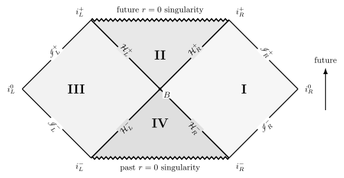
The maximal eternal Schwarzschild solution has right and left exteriors (I and III), a future black-hole region (II), and a past white-hole region (IV). Future points upward; solid diagonal boundaries are null, jagged horizontal boundaries are the spacelike $r=0$ curvature singularities, and each interior point represents a suppressed symmetry two-sphere. The compactified diagram is schematic and not to scale.

The canonical Schwarzschild conformal-diagram record explains the compactification and gives the full key to null, timelike, and spatial infinity.

The Einstein–Rosen bridge is spatial, not traversable

The reflection-symmetric slice $T_K=0$ has $U=-V=-X_K$ and

$$X_K^2=\left(\frac{r}{r_s}-1\right)e^{r/r_s}, \qquad r=r_s\left[1+W_0\!\left(\frac{X_K^2}{e}\right)\right].$$

It has two asymptotically flat ends, $X_K\to+\infty$ in I and $X_K\to-\infty$ in III, joined at $X_K=0$. The areal radius is not one-to-one on this slice: as signed proper distance $\ell$ increases from the left end, $r$ decreases from infinity to $r_s$ and then increases back to infinity toward the right end. Its induced spatial metric is

$$dl^2=\frac{dr^2}{1-r_s/r}+r^2d\Omega_2^2.$$

If $\ell$ is signed proper radial distance from the joining sphere, then

$$\left(\frac{dr}{d\ell}\right)^2=1-\frac{r_s}{r}, \qquad \frac{d^2r}{d\ell^2}=\frac{r_s}{2r^2}.$$

At $\ell=0$, therefore, $r=r_s$, $dr/d\ell=0$, and $d^2r/d\ell^2=1/(2r_s)\gt0$. The sphere is the unique minimum of the areal radius, with area $4\pi r_s^2$. The divergent coefficient of $dr^2$ at $r=r_s$ records the failure of $r$ to be a coordinate at this minimum; the signed coordinate $\ell$ and the spatial geometry are smooth there. This time-symmetric spatial connection is the Einstein–Rosen bridge described in Kruskal 1960, p. 1743 and Fig. 1 on p. 1744.

One equatorial section makes the minimum visible without changing the intrinsic geometry. Embed it as a surface of revolution in an auxiliary Euclidean three-space. Matching

$$dl_E^2=\left[1+\left(\frac{dz}{dr}\right)^2\right]dr^2+r^2d\phi^2$$

to the induced metric gives

$$\left(\frac{dz}{dr}\right)^2=\frac{r_s}{r-r_s}, \qquad z_\pm(r)=\pm2\sqrt{r_s(r-r_s)}, \qquad r\geq r_s.$$

Panel (b) below plots this exact isometric profile for one equatorial two-surface; compare it with the representative future-directed arrows in panel (a). The comparison is the important point: one spatial slice is connected, but the spacetime supplies no causal route through it from one exterior to the other.

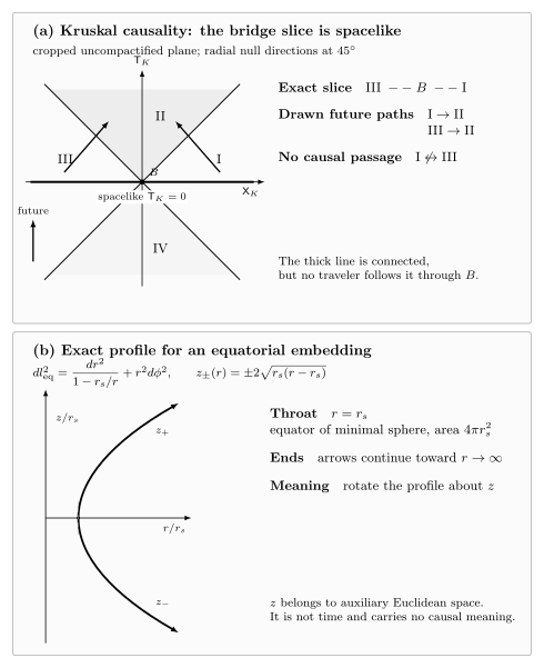
Panel (a) is a schematic, uncompactified Kruskal view: the exact spacelike $T_K=0$ slice joins exteriors III and I through the bifurcation sphere, while the two drawn horizon-crossing future causal curves enter Region II rather than the other exterior. Panel (b) is the exact, equal-scale auxiliary Euclidean surface-of-revolution profile $z_\pm(r)=\pm2\sqrt{r_s(r-r_s)}$ for one equatorial two-surface of that slice. Its throat circle is the equator of the minimal $r=r_s$ sphere, whose area is $4\pi r_s^2$; the plotted branches are cropped, and their arrowheads mark continuation to $r\to\infty$. The embedding is not the shape of four-dimensional spacetime and does not represent a traversable tunnel.

A bridge on one spacelike slice is not a causal tunnel. Any future-directed curve from I to III would have to change $V$ from positive to negative, contradicting $dV\geq0$; a future-directed curve from III to I would have to make $U$ decrease through zero, contradicting $dU\geq0$. A traveler who crosses a future horizon instead enters II and cannot avoid the future singular boundary. The noncommunication of the two exteriors is visible in Kruskal 1960, Fig. 2 on p. 1744 and p. 1745 and Reall 2013, § 12.6, printed p. 147, Open PDF.

Why maximal does not mean complete

The remaining finite Kruskal boundary is $r=0$, or $UV=1$. Since

$$UV=T_K^2-X_K^2,$$

its future and past branches are

$$T_K=+\sqrt{1+X_K^2}, \qquad T_K=-\sqrt{1+X_K^2}.$$

The normal to $T_K^2-X_K^2=1$ is timelike in the conformal radial metric, so each singular branch is spacelike. This causal label alone does not establish a physical singularity; curvature does:

$$R_{\mu\nu\rho\sigma}R^{\mu\nu\rho\sigma} =\frac{12r_s^2}{r^6} =\frac{48G^2M^2}{r^6} \longrightarrow\infty \quad\text{as}\quad r\to0.$$

The divergence excludes any $C^2$ Lorentzian extension through $r=0$. It also occurs at finite affine parameter. For a radial null geodesic with tangent $k^a$ and Killing energy $E=-\xi\cdot k\neq0$, normalized using an exterior, the null equation gives

$$\left(\frac{dr}{d\lambda}\right)^2=E^2, \qquad \lvert\Delta\lambda\rvert_{r_s\to0}=\frac{r_s}{\lvert E\rvert}.$$

Thus an ingoing ray reaches $r=0$ after a finite affine interval. The spacetime is geodesically incomplete.

There is no contradiction. Maximal analytic means that no regular analytic boundary remains through which this spacetime can be embedded as a proper open subset; it does not mean that every geodesic has infinite parameter length. Kruskal’s decisive step is exhaustive: every inextendible geodesic either reaches $r=0$ or continues for infinite affine parameter (proper time or proper length for non-null geodesics). A proper regular extension would instead supply a geodesic crossing its new boundary after finite parameter, which contradicts that alternative. Kruskal coordinates already cross the regular horizons, ordinary angular charts cover the poles of each sphere, and the remaining incomplete finite boundary has divergent curvature. The asymptotic conformal infinities are ideal endpoints rather than omitted finite-metric hypersurfaces. This is the classic argument of Kruskal 1960, pp. 1743–1745, Tables I–II and Figs. 1–2. Questions below $C^2$ regularity require different tools and are outside this page’s scope.

Eternal vacuum extension versus stellar collapse

The maximal extension answers a mathematical continuation question: what is the largest standard analytic Schwarzschild vacuum containing the static exterior? It does not say that both exteriors and the white hole arise when a star collapses. Reall’s comparison concerns the standard one-ended, asymptotically flat, spherically symmetric stellar-collapse model Reall 2013, §§ 12.5–12.6, printed pp. 141–148, Open PDF.

Feature	Eternal Kruskal vacuum	Standard one-ended spherical collapse
Field content	Vacuum everywhere with $r\gt0$	Matter in the star; Schwarzschild vacuum only outside it
Asymptotic ends	Two, Regions I and III	One
Past interior	White-hole region and past singularity	Regular stellar center before collapse
Bifurcation sphere	Present where past and future Killing horizons meet	Generically absent; the event horizon has a past endpoint in the regular region
Future black hole	Region II is eternal as part of the full solution	Forms during the global collapse history
What a late exterior determines	The local Schwarzschild geometry and mass $M$	Not the interior matter, past history, or global completion

The collapse conformal diagram shows how the matter region replaces the left exterior, white hole, and past singularity. This is why a horizon-penetrating coordinate system does not by itself select a collapse spacetime: the distinction lies in the matter, initial data, matching, and global domain. An event horizon is defined relative to an entire future and can have a past endpoint in a perfectly regular matter region; inside the star it need not be a locally distinguished surface $r=r_s$. The late-time exterior may be exactly Schwarzschild while leaving that history undetermined. The precise global definition is developed in Event Horizons as Global Boundaries; the next charged comparison begins with The Reissner–Nordström Solution.

Common pitfalls

Regular at one horizon does not mean maximal. Advanced and retarded Eddington–Finkelstein charts are individually smooth at one relevant horizon branch, but neither contains the bifurcation sphere or all four regions.

The two interiors are not duplicate coordinates. The $r\lt r_s$ part of the advanced chart is the future black-hole region II; the $r\lt r_s$ part of the retarded chart is the past white-hole region IV.

Region III is a distinct asymptotic end. It is not a second label for an event in Region I. No future-directed causal curve connects the two exteriors.

A spatial bridge is not a traversable wormhole. The $T_K=0$ slice connects two ends geometrically, but the four-dimensional causal cones forbid travel through it from one exterior to the other.

Maximal is not complete. The horizons are removable coordinate boundaries; $r=0$ is a curvature-singular boundary reached by some geodesics in finite parameter.

Eternal is not formed by collapse. A regular one-ended collapse spacetime can share the same late Schwarzschild exterior without containing Region III, Region IV, or the bifurcation sphere.

Exercises

1. Why a fourth region appears

Show that $H(x)=(x-1)e^x$ maps $x\gt0$ bijectively to $(-1,\infty)$ and invert the product relation with $W_0$. Then explain why adjoining the bifurcation sphere to the advanced and retarded patches requires Region III.

Solution

Since $H'(x)=xe^x\gt0$, the function is strictly increasing for $x\gt0$. Its limits are $\lim_{x\to0^+}H(x)=-1$ and $H(x)\to\infty$ as $x\to\infty$, so its image is $(-1,\infty)$. Writing $y=x-1$ gives

$$\frac{-UV}{e}=ye^y,$$

hence $y=W_0(-UV/e)$ and

$$r=r_s\left[1+W_0\!\left(-\frac{UV}{e}\right)\right], \qquad UV\lt1.$$

The advanced patch has $V\gt0$ and contains quadrants I and II. The retarded patch has $U\lt0$ and contains I and IV. Their union misses $U\gt0,V\lt0$, which is III, and neither chart contains the origin. Every open disk around $(0,0)$ intersects all four quadrants. Therefore a coordinate neighborhood of the regular bifurcation sphere cannot contain I, II, and IV while omitting III.

2. See the horizon pole cancel

Starting from $ds_{\mathrm{rad}}^2=-f\,du\,dv$, derive the Kruskal coefficient $A(r)$. Then compute $g_{UV}$ and the radial determinant at $r=r_s$. Why does this establish a local extension through the horizons but not maximality by itself?

Solution

The exponential definitions give

$$du=-2r_s\frac{dU}{U}, \qquad dv=2r_s\frac{dV}{V}.$$

Therefore

$$ds_{\mathrm{rad}}^2 =\frac{4r_s^2f}{UV}\,dU\,dV.$$

Writing $x=r/r_s$, one has $f=(x-1)/x$ and $UV=-(x-1)e^x$. Hence

$$ds_{\mathrm{rad}}^2 =-\frac{4r_s^2}{x}e^{-x}\,dU\,dV =-\frac{4r_s^3}{r}e^{-r/r_s}\,dU\,dV =-A(r)\,dU\,dV.$$

Because the symmetric cross term is $2g_{UV}\,dU\,dV$,

$$g_{UV}=g_{VU}=-\frac{A}{2}, \qquad \det g_{UV}=-\frac{A^2}{4}.$$

At the horizon, $A=4r_s^2/e$, so

$$g_{UV}=-\frac{2r_s^2}{e}, \qquad \det g_{UV}=-\frac{4r_s^4}{e^2}\neq0.$$

The continued metric is therefore smooth and nondegenerate in a neighborhood of either horizon. Maximality is a global claim: one must still include a neighborhood of the bifurcation sphere, examine all remaining boundaries, and rule out any further regular extension.

3. Causal monotonicity and non-traversability

Using $dU\geq0$ and $dV\geq0$ for future causal directions, prove that $r$ decreases in II and increases in IV. For a future-inextendible causal curve in II beginning at $U_0,V_0\gt0$, prove that $UV\to1$. Then rule out future-directed causal travel between I and III in either direction.

Solution

Let $P=UV$. Because $dr/dP\lt0$, it is enough to determine the sign of

$$dP=V\,dU+U\,dV.$$

In II, $U,V\gt0$, so every nonzero future causal displacement has $dP\gt0$ and hence $dr\lt0$. In IV, $U,V\lt0$, so $dP\lt0$ and $dr\gt0$.

Along the curve in II, $U\geq U_0$ and $V\geq V_0$. Since $UV\lt1$,

$$U\lt\frac1{V_0}, \qquad V\lt\frac1{U_0}.$$

Both monotone coordinates therefore have finite limits. Suppose their product tended to $P_\infty\lt1$. On a compact neighborhood of that putative endpoint, $A/r^2$ is bounded by a constant $C$. Causality gives

$$\lvert\dot\Omega\rvert^2 \leq C\dot U\dot V,$$

and the Cauchy–Schwarz inequality then bounds the total angular length by $\sqrt{C\,\Delta U\,\Delta V}$. The angular position also converges, so the curve has a regular endpoint in $\mathcal D\times S^2$ and can be extended. This contradicts future inextendibility. Consequently $UV\to1$ and $r\to0$.

Region I has $V\gt0$, whereas III has $V\lt0$. A curve from I to III would therefore have to decrease $V$, contrary to $dV\geq0$. Conversely, III has $U\gt0$ whereas I has $U\lt0$, so a curve from III to I would have to decrease $U$, contrary to $dU\geq0$.

4. The minimum-area sphere

On the $T_K=0$ slice, use the proper-distance equations to show that the bifurcation sphere is a strict local minimum of area. What is its area?

Solution

The area of a symmetry sphere is $\mathcal A=4\pi r^2$. At the throat, $r=r_s$ and $dr/d\ell=0$, so

$$\frac{d\mathcal A}{d\ell}=8\pi r\frac{dr}{d\ell}=0.$$

Differentiating once more gives

$$\frac{d^2\mathcal A}{d\ell^2} =8\pi\left[\left(\frac{dr}{d\ell}\right)^2 +r\frac{d^2r}{d\ell^2}\right].$$

At $r=r_s$, this equals $8\pi r_s[1/(2r_s)]=4\pi\gt0$. The sphere is therefore a strict local minimum, and its area is

$$\mathcal A_{\mathrm{throat}}=4\pi r_s^2=16\pi G^2M^2.$$

5. Finite affine parameter is not a coordinate failure

The radial part of the ingoing Eddington–Finkelstein metric is

$$ds^2=-\left(1-\frac{r_s}{r}\right)dv^2+2\,dv\,dr.$$

Show that curves with $v$ constant are radial null geodesics with $r$ an affine parameter. What happens at $r=r_s$ and at $r=0$?

Solution

For $dv=0$ and fixed angles, the line element vanishes, so the curves are null. Moreover, $g_{rr}=0$ and $g_{rv}=1$ are constant. The Christoffel formula therefore gives

$$\Gamma^a{}_{rr}=0,$$

so $k^a=(\partial_r)^a$ obeys $k^b\nabla_bk^a=0$. Any nonconstant affine-linear function of $r$ is an affine parameter; the future-directed ingoing orientation uses $-\partial_r$.

The geodesic crosses $r=r_s$ after a finite affine change with no metric or curvature singularity. It reaches $r=0$ after another finite affine change, but there the Kretschmann scalar diverges. The first endpoint was only a bad static coordinate boundary; the second is a genuine $C^2$ obstruction and makes the maximal spacetime incomplete.

References

• Kruskal, Martin D. “Maximal Extension of Schwarzschild Metric.” Physical Review 119, no. 5 (1960): 1743–1745. DOI: 10.1103/PhysRev.119.1743.
• Reall, Harvey S. General Relativity. Cambridge Part III lecture notes, 2013. Open PDF.
• Szekeres, Gy. “On the Singularities of a Riemannian Manifold.” Publicationes Mathematicae Debrecen 7, nos. 1–4 (1960): 285–301. DOI: 10.5486/PMD.1960.7.1-4.26. Publisher PDF.