Deriving the Schwarzschild Metric

The Schwarzschild metric follows from two ordinary differential equations on a connected static spherical patch. One equation makes the mass function constant; the other determines the redshift factor. After the time coordinate is normalized, the sole invariant parameter is the mass $M$. This page solves the reduced equations explicitly and keeps that calculation logically separate from Birkhoff’s theorem, which is the stronger statement that spherical vacuum symmetry itself produces an additional Killing field.

Required background. The Einstein Equation supplies the vacuum equation $G_{\mu\nu}=0$ and the contracted Bianchi identity used below.

Helpful background. The Riemann Curvature Tensor supports the invariant check; Exact Solutions of Einstein’s Equations explains how to specify a spacetime and its matter fields; Causality and Global Structure distinguishes this local derivation from global extension; Affine and Variational Geodesics supplies the conserved Killing energy and affine-parameter reasoning used in the final exercise.

Static spherical vacuum data and logical scope

Work in four-dimensional Einstein gravity with $\Lambda=0$ and $T_{\mu\nu}=0$. Each orbit of the rotation group is a round two-sphere. Its geometrically defined areal radius $r$ satisfies

$$\operatorname{Area}(S^2)=4\pi r^2.$$

On an open region where the spherical vacuum geometry is static, let $\xi$ be the static Killing field. Here static means more than time independent: $\xi$ is timelike and hypersurface orthogonal. Choose $t$ along its orbits, so $\xi=\partial_t$, and choose the constant-$t$ hypersurfaces orthogonal to $\xi$. This removes a $dt\,dr$ cross term rather than assuming it away.

Rotations and time translations leave the area of each symmetry sphere unchanged, so $r$ depends only on the remaining radial direction. Where $\nabla_\mu r$ is spacelike, it is nonzero and $r$ itself is a valid coordinate on the two-dimensional orbit space. Spherical and static symmetry then make every remaining metric coefficient a function of $r$ alone. Defining

$$e^{2\Phi(r)}=-g(\xi,\xi), \qquad A(r)=g^{\mu\nu}\nabla_\mu r\nabla_\nu r=g^{rr},$$

gives the most general metric in this gauge:

$$ds^2=-e^{2\Phi(r)}dt^2+\frac{dr^2}{A(r)}+r^2d\Omega_2^2, \qquad d\Omega_2^2=d\theta^2+\sin^2\theta\,d\phi^2.$$

It is useful to define a mass function $m(r)$ by

$$A(r)=1-\frac{2Gm(r)}{r}.$$

Because both $A=(\nabla r)^2$ and $r$ are geometrically defined, this equation defines $m$ geometrically: it is the Misner–Sharp mass in spherical symmetry. The static chart requires $A\gt0$, $e^{2\Phi}\gt0$, and $r\gt0$. It therefore does not cover a region where $\nabla r$ is timelike, a horizon where $A=0$, or a critical point of $r$.

The logical roles are worth fixing before any algebra:

Statement	Status on this page
A static, spherically symmetric vacuum patch admits the displayed areal-radius form.	Geometric consequence of the stated assumptions, followed by an areal-radius coordinate choice
The vacuum equations reduce that form to the one-parameter Schwarzschild family.	Derived below
A general spherically symmetric vacuum solution has the required extra Killing symmetry.	Birkhoff’s theorem; linked below, not proved by the ansatz

Carroll constructs the static areal-radius gauge in Carroll 2014, §5.1, printed pp. 193–195, then gives the reduced equations, time rescaling, mass identification, and the logically separate symmetry-enhancement argument in Carroll 2014, §5.1, pp. 195–197, and §5.2, pp. 197–204. His functions map to the present notation as $\alpha=\Phi$ and $e^{-2\beta}=A$. Keeping these two directions separate prevents a common circular argument.

The two independent radial equations

A prime denotes $d/dr$. To make the sign conventions traceable before the tensor result is used, the radial connection coefficients and two representative sphere-coupling coefficients are

$$\begin{gathered} \Gamma^t{}_{tr}=\Phi', \qquad \Gamma^r{}_{tt}=Ae^{2\Phi}\Phi', \qquad \Gamma^r{}_{rr}=-\frac{A'}{2A}, \\[3pt] \Gamma^r{}_{\theta\theta}=-Ar, \qquad \Gamma^\theta{}_{r\theta}=\Gamma^\phi{}_{r\phi}=\frac1r. \end{gathered}$$

Together with the intrinsic connection of the unit sphere, substituting these coefficients into the Ricci definition gives the mixed Einstein tensor

$$\begin{aligned} G^t{}_t &=\frac{rA'+A-1}{r^2} =-\frac{2Gm'}{r^2},\\ G^r{}_r &=\frac{2A\Phi'}{r}+\frac{A-1}{r^2},\\ G^\theta{}_\theta=G^\phi{}_\phi &=A\left(\Phi''+\Phi'^2+\frac{\Phi'}{r}\right) +\frac{A'}{2}\left(\Phi'+\frac{1}{r}\right). \end{aligned}$$

Spherical symmetry makes the two angular components equal, while staticity makes all off-diagonal components vanish. The contracted Bianchi identity means that only two of the three displayed equations are independent. We will solve the $tt$ and $rr$ equations and then check the angular equation directly.

The first vacuum equation is immediate:

$$G^t{}_t=0 \quad\Longrightarrow\quad m'(r)=0 \quad\Longrightarrow\quad m(r)=M$$

on the connected interval. More precisely, the exact spherical mass equation has no matter source in vacuum, so the Misner–Sharp mass cannot change from one symmetry sphere to the next. This statement does not assign a local energy density to the gravitational field; that field is already encoded in the geometry.

Set

$$f(r)=1-\frac{2GM}{r}.$$

The second equation then reads

$$0=G^r{}_r =\frac{2f\Phi'}{r}-\frac{2GM}{r^3}.$$

Solving for the derivative of the redshift potential gives two equivalent forms:

$$\Phi' =\frac{GM}{r(r-2GM)} =\frac{f'}{2f}.$$

Hence

$$\Phi(r)=\frac12\ln f(r)+\Phi_0, \qquad e^{2\Phi(r)}=C f(r), \qquad C=e^{2\Phi_0}\gt0.$$

The sign $C\gt0$ is required because the static Killing direction is timelike on this patch. At this stage the local metric is

$$ds^2=-C f(r)dt^2+f(r)^{-1}dr^2+r^2d\Omega_2^2.$$

Why the angular equation also vanishes

Invoking the Bianchi identity would be enough, but a direct check exposes any sign error in the reduction. Substitute $A=f$ and $\Phi'=f'/(2f)$ into the angular component. The terms proportional to $f'^2/f$ cancel, leaving

$$G^\theta{}_\theta =G^\phi{}_\phi =\frac{f''}{2}+\frac{f'}{r}.$$

For $f=1-2GM/r$,

$$f'=\frac{2GM}{r^2}, \qquad f''=-\frac{4GM}{r^3},$$

and therefore

$$G^\theta{}_\theta =-\frac{2GM}{r^3}+\frac{2GM}{r^3} =0.$$

Thus every component of $G^\mu{}_\nu$ vanishes. This calculation is also a useful diagnostic: solving only one radial equation would not be sufficient.

Normalization and the physical parameter

The constant $C$ is not a second gravitational charge. The coordinate change

$$t_\infty=\sqrt C\,t$$

removes it locally because $-Cf\,dt^2=-f\,dt_\infty^2$. If the patch belongs to a chosen asymptotically flat end, the notation $t_\infty$ is natural: select $\partial_{t_\infty}$ to be future-directed and require its norm to approach $-1$ there. Unit normalization fixes the magnitude of the Killing generator, while the spacetime time orientation fixes its remaining sign. The normalized metric is then

$$ds^2=-f(r)dt_\infty^2+f(r)^{-1}dr^2+r^2d\Omega_2^2, \qquad f(r)=1-\frac{2GM}{r}.$$

In the weak-field limit, $g_{tt}\simeq-(1+2\Phi_N)$, where $\Phi_N$ is the Newtonian potential. Since

$$g_{t_\infty t_\infty}=-1+\frac{2GM}{r},$$

one reads off $\Phi_N=-GM/r$. Thus $M$ is the Newtonian mass. The ADM calculation gives the same result rather than following from the weak-field comparison alone. The ADM energy–momentum hypotheses explain why the surface integral is geometric only after an admissible asymptotically Euclidean end, its decay, and its coordinate class have been specified.

Let $\gamma_{ij}$ be the induced metric on a constant-$t_\infty$ slice, let $\delta_{ij}$ be the Euclidean metric in asymptotically Cartesian coordinates, and set $p_{ij}=\gamma_{ij}-\delta_{ij}$. Because $dr=n_i\,dx^i$ for $n_i=x_i/r$, the spatial metric obeys the exact relation

$$\gamma_{ij}=\delta_{ij}+\bigl(f^{-1}-1\bigr)n_i n_j.$$

Expanding its smooth radial coefficient at infinity gives

$$\gamma_{ij} =\delta_{ij}+\frac{2GM}{r}n_i n_j+O(r^{-2}), \qquad p_{ij}=\frac{2GM}{r}n_i n_j+O(r^{-2}).$$

Here $f^{-1}-1=2GM/(r-2GM)$, so the displayed remainder and its first derivative have the falloff required by the ADM hypotheses. Since $p_{ij}=2GMx_ix_j/r^3+O(r^{-2})$ and $p_{jj}=2GM/r+O(r^{-2})$,

$$\partial_jp_{ij} =\frac{2GM}{r^2}n_i+O(r^{-3}), \qquad \partial_i p_{jj} =-\frac{2GM}{r^2}n_i+O(r^{-3}).$$

Consequently, using the leading Euclidean sphere normal and area element,

$$\begin{aligned} M_{\mathrm{ADM}} &=\frac{1}{16\pi G}\lim_{r\to\infty} \int_{S_r}(\partial_jp_{ij}-\partial_i p_{jj})n^i\,dS\\ &=\frac{1}{16\pi G}\int_{S^2}4GM\,d\Omega=M. \end{aligned}$$

Without an asymptotic end, $M$ remains the invariant Schwarzschild—or vacuum Misner–Sharp—parameter, but no preferred normalization of the Killing generator is supplied by the local geometry alone. Reall discusses the solution, its weak-field mass identification, and its chart boundary in Reall 2013, §12.1, pp. 131–133, Open PDF; his geometrized mass parameter is the length $GM$ in the notation used here.

The answer to the integration-constant question is therefore sharp: $M$ survives as a geometric parameter, $C$ is removed by normalizing time, and the angular equation contributes no third constant. At an asymptotically flat end with the stated normalization, the surviving parameter also equals $M_{\mathrm{ADM}}$. The diagram below places the mass and redshift equations in parallel. Follow the left lane to see why $M$ survives, the right lane to see why $C$ does not, and the dashed upper box to keep Birkhoff’s theorem outside the derivation.

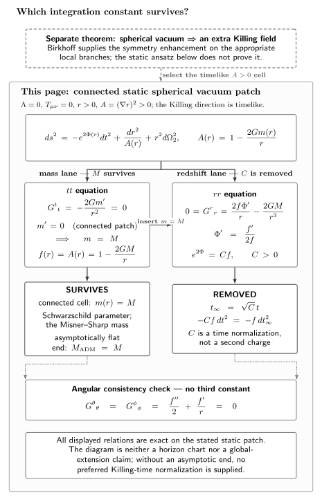
On a connected static spherical vacuum patch, $G^t{}_t=0$ gives $m'=0$ and hence one constant $M$, while $G^r{}_r=0$ gives $e^{2\Phi}=Cf$ with $C\gt0$. The angular equation checks the result but introduces no new constant. The rescaling $t_\infty=\sqrt C\,t$ removes $C$; if an asymptotically flat end supplies unit Killing normalization, the surviving $M$ equals $M_{\rm ADM}$. The derivation begins after staticity is assumed, so the schematic is neither a proof of Birkhoff’s theorem nor a horizon-extension diagram.

Curvature check and the three mass branches

We have checked every component of $G^\mu{}_\nu$. Its trace in four dimensions is $G^\mu{}_\mu=-R$, so vacuum gives $R=0$ and then $R_{\mu\nu}=G_{\mu\nu}+\tfrac12Rg_{\mu\nu}=0$. The Kretschmann invariant is

$$R_{\mu\nu\rho\sigma}R^{\mu\nu\rho\sigma} =\frac{48G^2M^2}{r^6}.$$

For the Schwarzschild family, this scalar detects the curvature blow-up at $r=0$ and remains finite as the positive-mass static chart approaches $r=2GM$; see Carroll 2014, §5.3, printed pp. 204–205, especially Eq. (5.50). Finiteness of one scalar is not, by itself, a general proof of regularity. Here the Schwarzschild coordinate atlas supplies the missing geometric evidence by constructing nondegenerate horizon-crossing coordinates.

The field equations themselves permit three branches:

Mass	Static-patch domain	Interpretation
$M\gt0$	$r\gt2GM$	Exterior Schwarzschild patch. At $r=2GM$, the scalar above is finite but the static chart ends.
$M=0$	$r\gt0$ in spherical coordinates	Minkowski spacetime. The apparent endpoint $r=0$ is a removable coordinate center after passing to Cartesian coordinates.
$M\lt0$	Every $r\gt0$	No positive-radius zero of $f$ and hence no Schwarzschild Killing horizon; $r=0$ is a curvature singularity not shielded by such a horizon.

For the positive-mass branch,

$$\lim_{r\to(2GM)^+}R_{\mu\nu\rho\sigma}R^{\mu\nu\rho\sigma} =\frac{3}{4G^4M^4},$$

which is finite for $M\ne0$. By contrast, the invariant diverges as $r\to0$ whenever $M\ne0$. The positive mass theorem can exclude the negative-mass branch only under its asymptotic, completeness, regularity, dimensional, and energy hypotheses; the singular negative-mass slice does not satisfy that complete regular setting, and the local vacuum equations alone do not impose $M\ge0$.

The Schwarzschild coordinate atlas constructs coordinates regular across the positive-mass horizon, and the maximal Schwarzschild extension studies the resulting global geometry. Bičák places the static chart within that wider exact-solution history in Bičák 2000, §§2.1–2.3, printed pp. 19–22, Open PDF; his Schwarzschild parameter is likewise a geometrized mass length.

Birkhoff’s theorem is a separate implication

The calculation began after assuming a static patch. Starting instead with an arbitrary spherically symmetric vacuum metric, the field equations imply an extra hypersurface-orthogonal Killing field on the appropriate local branches. That is the content of the vacuum Birkhoff theorem.

The distinction matters inside the positive-mass black hole, where $f=(\nabla r)^2\lt0$. The spacetime is still locally Schwarzschild, but the timelike-static areal-radius chart used here no longer applies: $r$ is timelike and the Birkhoff Killing field is spacelike. Horizons and critical points likewise require charts adapted to their own geometry. Consequently, this page proves neither global uniqueness nor that an astrophysical collapse spacetime contains all regions of the eternal extension.

To see how a matter field changes the same calculation, continue to the Reissner–Nordström solution. Its electromagnetic energy makes the spherical mass function vary with radius before asymptotic mass is identified, while the residual normalization of Killing time is removed in the same way.

Common pitfalls

Treating the ansatz as a proof of Birkhoff’s theorem. A static ansatz classifies metrics already known to be static. Birkhoff’s theorem supplies the missing implication from spherical vacuum symmetry to the extra Killing field, including branches not covered by this chart.

Counting $C$ as a second physical parameter. The positive constant in $g_{tt}=-Cf$ disappears under $t_\infty=\sqrt C\,t$. Boundary normalization chooses a representative Killing generator; it does not create a new charge.

Calling $r=2GM$ a curvature singularity. The inverse radial coefficient diverges in the static chart, while the Kretschmann scalar remains finite. That scalar alone is not a general regularity proof; the horizon-regular coordinates constructed in the atlas establish that the Schwarzschild geometry extends smoothly across this chart boundary.

Exercises

1. Recover the mass equation

Starting from $A=1-2Gm/r$, show that $(rA'+A-1)/r^2=-2Gm'/r^2$ and explain why vacuum makes $m$ constant on a connected interval.

Solution

Differentiate:

$$A'=-\frac{2Gm'}{r}+\frac{2Gm}{r^2}.$$

Therefore

$$rA'+A-1 =-2Gm'+\frac{2Gm}{r}-\frac{2Gm}{r} =-2Gm'.$$

The vacuum equation $G^t{}_t=0$ gives $m'=0$. A differentiable function with zero derivative is constant on each connected interval, so $m=M$ there.

2. Integrate the redshift equation

Integrate $\Phi'=GM/[r(r-2GM)]$ and explain why the resulting constant is not a second Schwarzschild charge.

Solution

Partial fractions give

$$\frac{GM}{r(r-2GM)} =\frac12\left(\frac{1}{r-2GM}-\frac{1}{r}\right).$$

Hence

$$\Phi=\frac12\ln\left(1-\frac{2GM}{r}\right)+\Phi_0,$$

and $e^{2\Phi}=e^{2\Phi_0}f=Cf$. The change $t_\infty=\sqrt{C}\,t$ removes $C$. At an asymptotically flat end, requiring $g(\partial_{t_\infty},\partial_{t_\infty})\to-1$ fixes the magnitude of the Killing generator, and choosing $\partial_{t_\infty}$ to be future-directed fixes its sign. Thus $C$ records a coordinate normalization, not an invariant charge.

3. Check the angular equation

Use $\Phi'=f'/(2f)$ to show directly that the angular Einstein equation becomes $f''/2+f'/r=0$ for $f=1-2GM/r$.

Solution

Differentiate once more:

$$\Phi''=\frac{f''}{2f}-\frac{f'^2}{2f^2}.$$

Substitution into

$$G^\theta{}_\theta =f\left(\Phi''+\Phi'^2+\frac{\Phi'}{r}\right) +\frac{f'}{2}\left(\Phi'+\frac1r\right)$$

produces three coefficients of $f'^2/f$: $-1/2$, $+1/4$, and $+1/4$. They cancel, leaving

$$G^\theta{}_\theta=\frac{f''}{2}+\frac{f'}{r}.$$

Since $f'=2GM/r^2$ and $f''=-4GM/r^3$, the two terms are $-2GM/r^3$ and $+2GM/r^3$. Their sum vanishes.

4. Recover the ADM mass

Let $p_{ij}=2GMn_i n_j/r+O(r^{-2})$ with $n_i=x_i/r$. Show that

$$(\partial_jp_{ij}-\partial_i p_{jj})n^i =\frac{4GM}{r^2}+O(r^{-3}),$$

and use the ADM surface integral to recover $M_{\mathrm{ADM}}=M$.

Solution

The leading perturbation can be written as

$$p_{ij}=2GM\frac{x_i x_j}{r^3}.$$

Differentiating and summing over $j$ gives

$$\begin{aligned} \partial_jp_{ij} &=2GM\,\partial_j\left(\frac{x_i x_j}{r^3}\right) =\frac{2GM}{r^2}n_i,\\ p_{jj}&=\frac{2GM}{r}, \qquad \partial_i p_{jj}=-\frac{2GM}{r^2}n_i. \end{aligned}$$

The omitted $O(r^{-2})$ metric terms contribute only $O(r^{-3})$ to the differentiated integrand. Contracting with the Euclidean unit normal and using $dS=r^2d\Omega$ at leading order therefore gives

$$\begin{aligned} M_{\mathrm{ADM}} &=\frac{1}{16\pi G}\lim_{r\to\infty} \int_{S_r}(\partial_jp_{ij}-\partial_i p_{jj})n^i\,dS\\ &=\frac{1}{16\pi G}\int_{S^2}4GM\,d\Omega=M. \end{aligned}$$

This calculation identifies the local constant with ADM mass only because an admissible asymptotically flat end and its unit time normalization have been supplied.

5. Classify the mass branches

For $M\gt0$, $M=0$, and $M\lt0$, determine where $f\gt0$, whether $f$ has a positive-radius zero, and whether $r=0$ is a curvature singularity.

Solution

If $M\gt0$, then $f\gt0$ for $r\gt2GM$ and $f=0$ at $r=2GM$. The invariant $48G^2M^2/r^6$ is finite at that zero, and a horizon-regular chart establishes that it is a static-chart boundary rather than a curvature singularity. The invariant diverges at $r=0$.

If $M=0$, then $f=1$ and the curvature invariant vanishes. The metric is Minkowski spacetime in spherical coordinates, whose origin can be added smoothly in Cartesian coordinates.

If $M\lt0$, write $M=-|M|$. Then $f=1+2G|M|/r\gt0$ for every $r\gt0$, so there is no positive-radius horizon. The curvature invariant still diverges at $r=0$.

6. Show that negative-mass Schwarzschild is naked

On the full asymptotically flat domain $r\gt0$ with $M\lt0$, set $a=2G|M|$ and consider a future-directed outgoing radial null geodesic with affine parameter $\lambda$.

1. Use its conserved Killing energy $E$ and the null condition to show that $dr/d\lambda=+E$. Prove that the geodesic has a past endpoint at $r=0$ after a finite affine interval.
2. Integrate $dt_\infty/dr=1/f$ by introducing a tortoise coordinate $r_*$. Show that the retarded coordinate $u=t_\infty-r_*$ is constant along the outgoing ray and has a finite one-sided value as $r\to0^+$.
3. Explain why the affine result, together with the ray’s arrival at future null infinity, establishes nakedness. Why is finite Schwarzschild coordinate time only supplementary evidence?

Solution

Let $k^\mu=dx^\mu/d\lambda$ be the geodesic tangent. Its conserved Killing energy is

$$E=-g(\partial_{t_\infty},k) =f\frac{dt_\infty}{d\lambda}\gt0.$$

The null condition then gives

$$0=-f\left(\frac{dt_\infty}{d\lambda}\right)^2 +f^{-1}\left(\frac{dr}{d\lambda}\right)^2, \qquad \frac{dr}{d\lambda}=+E$$

for the outgoing family. Thus an outgoing geodesic beginning at any $\varepsilon\gt0$ reaches every larger radius, with $r=\varepsilon+E(\lambda-\lambda_0)$. Define

$$\lambda_s=\lambda_0-\frac{\varepsilon}{E}, \qquad r=E(\lambda-\lambda_s).$$

Running the solution backward reaches $r=0$ at the finite affine value $\lambda_s$; because the curvature diverges there, the geodesic has no continuation through that endpoint in the Schwarzschild spacetime. To see its supplementary behavior in the static coordinates, the same geodesic obeys

$$\frac{dt_\infty}{dr}=\frac{1}{f}=\frac{r}{r+a}.$$

Its coordinate-time lapse from $r=\varepsilon$ to any fixed $R\gt0$ is

$$\Delta t_\infty =R-\varepsilon-a\ln\left(\frac{R+a}{\varepsilon+a}\right),$$

which remains finite as $\varepsilon\to0^+$. Equivalently, the retarded coordinate

$$u=t_\infty-r_*, \qquad r_*=r-a\ln\left(1+\frac{r}{a}\right)$$

is constant along the outgoing family, while $r_*$ has a finite one-sided limit at $r=0$ and grows without bound as $r\to\infty$. In the standard conformal completion of this asymptotically flat domain, the same past-incomplete rays reach future null infinity $\mathscr I^+$ at fixed finite $u$. In the boundary sense, the singular endpoint therefore lies in the causal past of $\mathscr I^+$: this affine statement, rather than coordinate-time finiteness by itself, is the precise reason negative-mass Schwarzschild is naked. The claim uses the full $r\gt0$ asymptotically flat domain, not merely the local field-equation calculation.

References

• Bičák, Jiří. “Selected Solutions of Einstein’s Field Equations: Their Role in General Relativity and Astrophysics.” In Einstein’s Field Equations and Their Physical Implications, edited by Bernd G. Schmidt, Lecture Notes in Physics 540, 1–126. Springer, 2000. DOI; Open PDF.
• Carroll, Sean M. Spacetime and Geometry: An Introduction to General Relativity. Pearson New International Edition. Pearson Education Limited, 2014. Author’s book page.
• Reall, Harvey S. General Relativity. Cambridge Part III lecture notes, 2013. Open PDF.