Invariants, Singularities, and Controlled Limits

The Reissner–Nordström solution gives us an exact metric and electromagnetic field; this page asks what coordinate-independent measurements say about them. Curvature invariants diverge at the central endpoint but remain finite at every positive horizon radius. That contrast is decisive evidence for a central scalar-curvature singularity, while the horizon-crossing charts on the preceding page supply the separate proof that the positive roots are smooth Killing horizons. The same calculations also reveal why neutral, flat, extremal, and near-horizon limits answer different questions unless we state what is held fixed.

Required background. The Einstein Equation supplies the vacuum and electrovac field equations.

Helpful background. The Riemann Curvature Tensor supplies the contractions used below; Electromagnetism with Differential Forms explains the two-form $F$, wedge products, and the form version of Maxwell’s equations; The Hodge Dual in Lorentzian Signature fixes the metric- and orientation-sensitive signs behind ${*F}$; Exact Solutions of Einstein’s Equations explains how invariants help characterize exact solutions; Causality and Global Structure distinguishes scalar blowup from global inextendibility; Affine and Variational Geodesics supplies complementary incompleteness tests.

The invariant profile of the spherical black holes

On the domain $r>0$, write the Schwarzschild and dyonic Reissner–Nordström families together as

$$ds^2=-f(r)\,dt^2+\frac{dr^2}{f(r)}+r^2d\Omega_2^2, \qquad f=1-\frac{2m}{r}+\frac{q^2}{r^2},$$ $$F=\frac{Q_e}{r^2}\,dr\wedge dt +Q_m\sin\theta\,d\theta\wedge d\phi, \qquad m=GM, \qquad q\equiv\sqrt{G(Q_e^2+Q_m^2)}\geq0.$$

We take $m>0$ unless the flat limit is stated explicitly. Thus $q^2=G(Q_e^2+Q_m^2)$, while the nonnegative symbol $q$ denotes the charge magnitude in geometrized units. The coordinate $r$ has an invariant meaning: every symmetry orbit has area $4\pi r^2$, so $r$ is the areal radius, not merely a chart label. In geometrized dimensions,

$$[m]=[q]=[r]=L,$$

and every quadratic curvature contraction below has dimension $L^{-4}$. This is a quick error detector: a term such as $m^2/r^6$ has the right dimension, whereas $m/r^6$ would not.

A scalar polynomial curvature invariant is formed by contracting the curvature tensor and its algebraic descendants until no indices remain. Define

$$S\equiv R_{\mu\nu}R^{\mu\nu}, \qquad K\equiv R_{\mu\nu\rho\sigma}R^{\mu\nu\rho\sigma}, \qquad W\equiv C_{\mu\nu\rho\sigma}C^{\mu\nu\rho\sigma}.$$

Here $K$ is the Kretschmann scalar, $S$ measures the Ricci part, and $W$ measures the trace-free conformal or tidal part. These are Lorentzian contractions, not positive-definite Euclidean norms in a general spacetime. Their special nonnegative forms in this family should not be silently generalized.

The Maxwell stress tensor is trace-free in four dimensions. Tracing Einstein’s equation therefore gives $R=0$—not because the charged spacetime is vacuum, but because its matter source has zero trace. Direct contraction gives

$$R=0, \qquad S=\frac{4q^4}{r^8},$$

and

$$K =\frac{48m^2}{r^6}-\frac{96mq^2}{r^7} +\frac{56q^4}{r^8}.$$

The four-dimensional algebraic decomposition of the Riemann tensor supplies an independent cross-check:

$$K=W+2S-\frac{1}{3}R^2.$$

Since $R=0$ here,

$$W=K-2S =\frac{48(mr-q^2)^2}{r^8} =48\left(\frac{m}{r^3}-\frac{q^2}{r^4}\right)^2.$$

The expression for $K$ is the $a=0$ specialization of Henry 2000, arXiv:astro-ph/9912320v1, PDF p. 6, and the Weyl result agrees with Herrera, Santos, and Skea 2003, § 3, arXiv:gr-qc/0306005v1, PDF pp. 4–5, Eqs. (10)–(14).

The formulas separate three physically different statements:

Locus or limit	Ricci square $S$	Kretschmann scalar $K$	Weyl square $W$	What follows
Any fixed positive radius, including $r=r_\pm>0$	Finite	Finite	Finite	No scalar-curvature obstruction occurs there; a regular chart is still needed to prove horizon smoothness.
Charged centre, $q\ne0$ and $r\to0$	$4q^4/r^8$	$56q^4/r^8$ to leading order	$48q^4/r^8$ to leading order	The endpoint is a scalar-curvature singularity.
Schwarzschild centre, $q=0$ and $r\to0$	$0$	$48m^2/r^6$	$48m^2/r^6$	Vacuum Ricci curvature vanishes, but tidal curvature still diverges.
Extremal horizon, $q^2=m^2$ and $r=m$	$4/m^4$	$8/m^4$	$0$	The horizon is curved and nonvacuum even though its Weyl tensor vanishes pointwise.

For $m,q>0$, the Weyl expression also vanishes on the sphere

$$r_C=\frac{q^2}{m}.$$

In the subextremal regime $0<q<m$, one can check $r_-<r_C<r_+$. At $r_C$, $S>0$ and $K=2S>0$: the Weyl part vanishes, but the spacetime is not flat. This spherically symmetric family is generically Petrov type D; its explicit Weyl components share the factor $mr-q^2$, so the Weyl tensor vanishes and the Petrov type degenerates to O on that sphere. A vanishing value of the single contraction $W$ would not justify the same conclusion in a generic Lorentzian spacetime.

The following exact plot makes the three special radii hard to confuse. Inspect the upper panel for finiteness at both roots and central divergence; then inspect the lower panel at the Weyl-zero sphere.

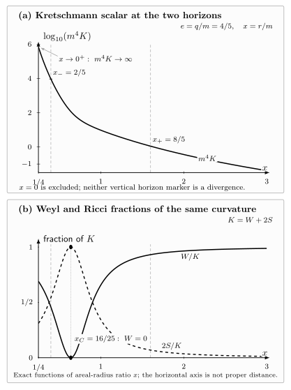
For the representative subextremal value $e=q/m=4/5$ and $x=r/m$, the upper panel plots $\log_{10}(m^4K)$ on $x>0$. The exact horizons $x_-=2/5$ and $x_+=8/5$ have finite curvature, whereas $K$ diverges toward the excluded centre $x=0$. The lower panel uses $W/K+2S/K=1$: at $x_C=e^2=16/25$, $W/K=0$ while $2S/K=1$, so the Weyl-free sphere remains curved. Every curve is quantitative in the displayed normalized coordinates; this is neither a causal diagram nor a proper-distance plot.

Electromagnetic invariants and the hidden duality angle

On any static component, where $f>0$, the natural orthonormal coframe gives the radial field components

$$F=-\frac{Q_e}{r^2}e^0\wedge e^1 +\frac{Q_m}{r^2}e^2\wedge e^3.$$

That coframe degenerates at a horizon and is unavailable in a region where $f<0$. The contractions obtained from it are scalars, however, so the formulas below extend across every regular horizon when evaluated in a regular chart.

With the site’s orientation, this gives two independent quadratic electromagnetic scalars,

$$F_{\mu\nu}F^{\mu\nu}=\frac{2(Q_m^2-Q_e^2)}{r^4}, \qquad F_{\mu\nu}{*F}^{\mu\nu}=+\frac{4Q_eQ_m}{r^4}.$$

The plus sign in the pseudoscalar is orientation-dependent; reversing the spacetime orientation reverses that sign. Squaring and adding removes the duality angle:

$$\left(F_{\mu\nu}F^{\mu\nu}\right)^2 +\left(F_{\mu\nu}{*F}^{\mu\nu}\right)^2 =\frac{4(Q_e^2+Q_m^2)^2}{r^8}.$$

Consequently, Einstein’s equation yields the useful electromagnetic–curvature bridge

$$S=G^2\left[ \left(F_{\mu\nu}F^{\mu\nu}\right)^2 +\left(F_{\mu\nu}{*F}^{\mu\nu}\right)^2 \right] =\frac{4q^4}{r^8}.$$

In the adopted Gaussian normalization, $\sqrt G\,F_{\hat a\hat b}$ has dimension $L^{-1}$, so this equation again has dimension $L^{-4}$.

Let $Q=\sqrt{Q_e^2+Q_m^2}$ and parameterize a nonzero field by

$$Q_e=Q\cos\alpha, \qquad Q_m=Q\sin\alpha.$$

Then the electromagnetic pair is proportional to $(-\cos2\alpha,\sin2\alpha)$, while the metric depends only on $Q^2$. The pair therefore determines $\alpha$ only modulo $\pi$: the shift $\alpha\mapsto\alpha+\pi$ sends $F\mapsto-F$ but leaves both quadratic scalars unchanged. Geometry alone forgets the entire continuous duality angle. This is why specifying an exact solution requires the matter field as well as the line element.

Controlled limits require held-fixed data

A limit is a comparison rule between members of a family. The phrase “take $q\to0$” is incomplete until the points, coordinates, and normalizations being compared are specified.

Limit	Held fixed	Result	Important qualification
Neutral	$m>0$ and a fixed $r>0$	$S\to0$ and $K,W\to48m^2/r^6$	Static metric components converge away from $r=2m$; a common horizon-regular chart gives smooth local convergence through the outer horizon.
Joint flat	A fixed point with $r>0$ while $m,q\to0$	All curvature and electromagnetic invariants vanish and the metric tends locally to Minkowski	The complete Minkowski manifold also fills in its regular centre, which is absent from every nontrivial member’s $r>0$ domain.
Extremal parameter	$m>0$, a fixed radius $r>m$ (hence exterior for $q$ sufficiently near $m$), fixed duality angle $\alpha$, and $q\uparrow m$ through subextremal values $0\leq q<m$	The two subextremal roots coalesce at $r=m$; the metric, invariants, and $F$ converge pointwise away from chart boundaries	Without fixed $\alpha$, $q^2\to m^2$ controls the geometry but not $F$; this limit also does not magnify the throat.
Extremal throat blow-up	First set $q^2=m^2$, then hold $(\tau,y,\theta,\phi)$ fixed as $\lambda\to0^+$	A finite $\mathrm{AdS}_2\times S^2$ metric and uniform electromagnetic field survive	Each fixed bounded $y$-window blows up a shrinking parent neighborhood; this is not substitution at one sphere.

The neutral limit becomes dramatically nonuniform if the observation point moves with the inner root. At fixed $m>0$,

$$r_-=m-\sqrt{m^2-q^2} =\frac{q^2}{m+\sqrt{m^2-q^2}} =\frac{q^2}{2m}+\frac{q^4}{8m^3} +O\!\left(\frac{q^6}{m^5}\right).$$

Thus $r_-$ approaches the singular centre as $q\to0$, and the invariant values along this moving sequence grow rather than approach a fixed-radius Schwarzschild value:

$$S(r_-)\sim\frac{1024m^8}{q^{12}}, \qquad K(r_-)\sim\frac{5120m^8}{q^{12}}, \qquad W(r_-)\sim\frac{3072m^8}{q^{12}}.$$

There is no contradiction. “Fixed $r>0$” and “follow $r_-(q)$” select different sequences of spacetime points.

At exact extremality, $q^2=m^2$ with $m>0$, the double horizon lies at $r=m$ and

$$S\big|_{r=m}=\frac{4}{m^4}, \qquad K\big|_{r=m}=\frac{8}{m^4}, \qquad W\big|_{r=m}=0.$$

These values will reappear from the throat geometry without referring back to the parent coordinates.

Blowing up the extremal throat

Set $q^2=m^2$ with $m>0$, introduce dimensionless coordinates $y$ and $\tau$ by

$$r=m(1+\lambda y), \qquad t=\frac{m}{\lambda}\tau,$$

and take $\lambda\to0^+$ while $(\tau,y,\theta,\phi)$ remain fixed. For every $\lambda>0$, the full range $y>0$ maps onto the entire exterior $r>m$. What shrinks is the image of each fixed bounded $y$-window: its radial width is $O(\lambda)$ and it approaches the horizon. There is no coordinate transformation at $\lambda=0$; the limit retains the leading geometry seen under progressively greater magnification.

The required cancellation is exact:

$$f=\left(1-\frac{m}{r}\right)^2 =\left(\frac{\lambda y}{1+\lambda y}\right)^2, \qquad dr=m\lambda\,dy.$$

Each metric term can now be followed separately:

$$\begin{aligned} -f\,dt^2 &=-m^2\frac{y^2}{(1+\lambda y)^2}\,d\tau^2,\\ f^{-1}dr^2 &=m^2\frac{(1+\lambda y)^2}{y^2}\,dy^2,\\ r^2d\Omega_2^2 &=m^2(1+\lambda y)^2d\Omega_2^2. \end{aligned}$$

Therefore

$$ds^2_{\mathrm{NH}} =m^2\left(-y^2d\tau^2+\frac{dy^2}{y^2}+d\Omega_2^2\right).$$

The two-form—not merely the metric—has a controlled limit:

$$\frac{Q_e}{r^2}\,dr\wedge dt =\frac{Q_e}{(1+\lambda y)^2}\,dy\wedge d\tau,$$

so

$$F_{\mathrm{NH}} =Q_e\,dy\wedge d\tau +Q_m\sin\theta\,d\theta\wedge d\phi, \qquad m^2=G(Q_e^2+Q_m^2).$$

The usual electric potential looks divergent only because of a gauge constant:

$$A_{\mathrm{el}} =-\frac{Q_e}{\lambda(1+\lambda y)}\,d\tau.$$

Adding the exact one-form $d(Q_e\tau/\lambda)$ gives

$$A'_{\mathrm{el}} =\frac{Q_e y}{1+\lambda y}\,d\tau \longrightarrow Q_e y\,d\tau,$$

whose exterior derivative is the electric term in $F_{\mathrm{NH}}$. The field strength was regular all along; the subtracted divergence was pure gauge.

On the exterior patch $y>0$, use the orthonormal coframe

$$e^0=my\,d\tau, \qquad e^1=m\frac{dy}{y}, \qquad e^2=m\,d\theta, \qquad e^3=m\sin\theta\,d\phi.$$

Then

$$F_{\mathrm{NH}} =-\frac{Q_e}{m^2}e^0\wedge e^1 +\frac{Q_m}{m^2}e^2\wedge e^3,$$

so the physical electric and magnetic components are constant. The first factor has sectional curvature $k_{\mathrm{AdS}_2}=-1/m^2$, while the sphere has $k_{S^2}=+1/m^2$. For a two-dimensional constant-curvature factor, $R=2k$, $R_{ab}R^{ab}=2k^2$, and $R_{abcd}R^{abcd}=4k^2$. Adding the two product factors gives

$$R=0, \qquad S=\frac{4}{m^4}, \qquad K=\frac{8}{m^4}, \qquad W=K-2S=0.$$

These are exactly the invariant values at the extremal horizon. Here conformal flatness does not follow from the single scalar $W=0$ alone. For a direct product of two-dimensional constant-curvature factors with curvatures $k_1$ and $k_2$, the purely factor components of the four-dimensional Weyl tensor are proportional to $(k_1+k_2)/3$, and the mixed components are proportional to $-(k_1+k_2)/6$. Because $k_{\mathrm{AdS}_2}+k_{S^2}=0$, every Weyl component vanishes. The throat is therefore conformally flat while its Ricci curvature is nonzero.

Writing $z=1/y$ turns the two-dimensional part into $m^2(-d\tau^2+dz^2)/z^2$. Thus $y\to\infty$ is the timelike conformal boundary of this Poincaré patch, while $y=0$ is its Poincaré horizon. The scaling establishes only this local patch of $\mathrm{AdS}_2\times S^2$. Its standard simply connected analytic extension is $\widetilde{\mathrm{AdS}}_2\times S^2$, conventionally called Bertotti–Robinson; the scaling alone does not select among alternative global identifications.

The metric limit is the $a=0$ specialization of Bardeen and Horowitz 1999, § 4, printed p. 12, Eqs. (4.1)–(4.2), arXiv:hep-th/9905099v1 PDF. The constant-field product solution appears in Bertotti 1959, printed pp. 1331–1333, especially Eqs. (6) and (16)–(17), and the extremal internal infinity and Robinson–Bertotti asymptotics are discussed in Bičák 2000, § 3.2, printed p. 39, arXiv:gr-qc/0004016v1 PDF. See Near-Horizon Scaling Limits for the general blow-up construction and Nariai and Bertotti–Robinson Geometries for the product-space comparison.

Common pitfalls

Mistaking $R=0$ for vacuum. The Maxwell field is nonzero and $R_{\mu\nu}$ is nonzero. Only the trace vanishes because the four-dimensional Maxwell stress tensor is trace-free.

Calling a finite-invariant root regular without checking a chart. Finite scalar polynomial invariants rule out one kind of singularity, but parallelly propagated curvature-component blow-up, distributional curvature, and quasiregular or quotient singularities may escape that test. For Reissner–Nordström, the regular advanced or retarded chart and its nondegenerate inverse supply the missing local horizon check.

Inferring flatness from $W=0$. A single vanishing Lorentzian contraction does not generally imply a vanishing tensor, and a vanishing Weyl tensor does not imply a vanishing Ricci tensor. At $r_C$ and in the extremal throat, the explicit algebraic calculation establishes $C_{\mu\nu\rho\sigma}=0$, but $S$ and $K$ remain positive.

Substituting $r=m$ and calling the result a throat. Substitution gives a degenerate induced expression at one coordinate sphere. The throat appears only after the simultaneous radial and time blow-up that keeps every metric term finite.

Treating all approaches to a parameter endpoint as equivalent. Fixed-$r$ neutral convergence is compatible with curvature divergence along $r_-(q)$ because these limits follow different points. Always name the held-fixed data before simplifying a limiting formula.

Asking scalar divergence to settle every extension problem. $K\to\infty$ rules out a curvature-bounded $C^2$ extension across the approached endpoint. It does not, by itself, classify weaker extensions, geodesic completeness, causal boundaries, or the global origin of the spacetime.

Exercises

1. From Maxwell stress to Ricci curvature

In an orthonormal frame, let $E=Q_e/r^2$ and $B=Q_m/r^2$. Show that the mixed Maxwell stress tensor has eigenvalues proportional to $(-u,-u,u,u)$ with $u=(E^2+B^2)/(8\pi)$, and use Einstein’s equation to recover $S=4q^4/r^8$.

Solution

With $\eta_{\hat a\hat b}=\operatorname{diag}(-1,1,1,1)$,

$$\begin{aligned} T_{\hat a\hat b} &=\frac{1}{4\pi}\left( F_{\hat a\hat c}F_{\hat b}{}^{\hat c} -\frac14\eta_{\hat a\hat b}F_{\hat c\hat d}F^{\hat c\hat d} \right),\\ F_{\hat c\hat d}F^{\hat c\hat d} &=2(B^2-E^2),\\ T_{\hat0\hat0} &=\frac{E^2+B^2}{8\pi}=u, \qquad T_{\hat1\hat1}=-\frac{E^2+B^2}{8\pi}=-u,\\ T_{\hat2\hat2}&=T_{\hat3\hat3}=u. \end{aligned}$$

Raising the first index changes only the temporal sign. The tensor is trace-free, and Einstein’s equation then gives

$$\begin{aligned} T^{\hat a}{}_{\hat b}=\operatorname{diag}(-u,-u,u,u), &\qquad T^{\hat a}{}_{\hat a}=0,\\ R^{\hat a}{}_{\hat b}&=8\pi G T^{\hat a}{}_{\hat b},\\ S=R^{\hat a}{}_{\hat b}R^{\hat b}{}_{\hat a} &=4(8\pi G u)^2 =4G^2(E^2+B^2)^2 =\frac{4G^2(Q_e^2+Q_m^2)^2}{r^8} =\frac{4q^4}{r^8}. \end{aligned}$$

2. Decomposition, the Weyl-free sphere, and extremality

Use the four-dimensional curvature decomposition to derive $W=K-2S$ for this electrovac family. Find the positive radius at which $W=0$, prove that it lies strictly between $r_-$ and $r_+$ when $0<q<m$, and evaluate $(S,K,W)$ at the extremal horizon.

Solution

Because $R=0$, the identity $K=W+2S-R^2/3$ gives

$$W=K-2S=\frac{48(mr-q^2)^2}{r^8}.$$

For $m,q>0$, this vanishes at $r_C=q^2/m$. Put $s=\sqrt{m^2-q^2}$, so $r_\pm=m\pm s$ and $q^2=m^2-s^2$. Then

$$r_C-r_-=\frac{s(m-s)}{m}>0, \qquad r_+-r_C=\frac{s(m+s)}{m}>0.$$

At extremality $q^2=m^2$ and $r=m$,

$$S=\frac{4}{m^4}, \qquad K=\frac{48-96+56}{m^4}=\frac{8}{m^4}, \qquad W=K-2S=0.$$

3. Recovering the duality angle

Set $Q_e=Q\cos\alpha$ and $Q_m=Q\sin\alpha$. Rewrite the two electromagnetic invariants in terms of $Q$ and $2\alpha$. Explain exactly which ambiguity remains and why the metric has a larger ambiguity.

Solution

Substitution gives

$$F_{\mu\nu}F^{\mu\nu} =-\frac{2Q^2}{r^4}\cos2\alpha, \qquad F_{\mu\nu}{*F}^{\mu\nu} =\frac{2Q^2}{r^4}\sin2\alpha.$$

For fixed orientation and $Q\ne0$, the ordered pair determines $2\alpha$ modulo $2\pi$, hence $\alpha$ modulo $\pi$. The remaining shift sends $(Q_e,Q_m)$ to $(-Q_e,-Q_m)$ and $F$ to $-F$. The metric depends only on $Q^2$, so it is unchanged under every continuous electric–magnetic duality rotation, not just the sign reversal.

4. A nonuniform neutral limit

At fixed $m>0$, expand $r_-$ through order $q^4$ as $q\to0$. Use only the leading term to derive the leading asymptotic behavior of $S(r_-)$, $K(r_-)$, and $W(r_-)$.

Solution

Rationalizing the root gives

$$r_-=\frac{q^2}{m+\sqrt{m^2-q^2}} =\frac{q^2}{2m}+\frac{q^4}{8m^3} +O\!\left(\frac{q^6}{m^5}\right).$$

Hence $r_-^{-8}\sim(2m/q^2)^8$. Direct substitution yields

$$S(r_-)\sim4q^4\left(\frac{2m}{q^2}\right)^8 =\frac{1024m^8}{q^{12}}.$$

For the Weyl square, $mr_--q^2\sim-q^2/2$, so

$$W(r_-)\sim48\frac{q^4}{4} \left(\frac{2m}{q^2}\right)^8 =\frac{3072m^8}{q^{12}}.$$

Finally $K=W+2S\sim5120m^8/q^{12}$. The divergence occurs because the sampled radius itself tends to zero.

5. The throat metric, field, and missing time rescaling

Carry out the extremal scaling for all metric terms and for the electric part of $F$. Then repeat the pullback with $r=m(1+\lambda y)$ but with the original $t$ held fixed. What tensor remains as $\lambda\to0^+$?

Solution

With $t=m\tau/\lambda$,

$$-fdt^2\to-m^2y^2d\tau^2, \qquad f^{-1}dr^2\to m^2\frac{dy^2}{y^2}, \qquad r^2d\Omega_2^2\to m^2d\Omega_2^2.$$

Moreover,

$$\frac{Q_e}{r^2}\,dr\wedge dt =\frac{Q_e}{(1+\lambda y)^2}\,dy\wedge d\tau \longrightarrow Q_e\,dy\wedge d\tau.$$

If $t$ is not rescaled, then $-fdt^2\to0$, while the radial and angular terms still approach

$$m^2\frac{dy^2}{y^2}+m^2d\Omega_2^2.$$

This is a rank-three degenerate tensor, not a Lorentzian spacetime metric. The missing $1/\lambda$ time magnification is precisely what preserves the temporal direction in the throat limit.

The extremal relation $q=m$ becomes the balance condition for several centres on Majumdar–Papapetrou Multi-Centre Equilibria.

References

• Bardeen, James M., and Gary T. Horowitz. “The Extreme Kerr Throat Geometry: A Vacuum Analog of AdS₂ × S².” Physical Review D 60, no. 10 (1999): 104030. DOI: 10.1103/PhysRevD.60.104030. Open PDF, arXiv:hep-th/9905099v1.
• Bertotti, Bruno. “Uniform Electromagnetic Field in the Theory of General Relativity.” Physical Review 116, no. 5 (1959): 1331–1333. DOI: 10.1103/PhysRev.116.1331.
• Bičák, Jiří. “Selected Solutions of Einstein’s Field Equations: Their Role in General Relativity and Astrophysics.” In Einstein’s Field Equations and Their Physical Implications, edited by Bernd G. Schmidt, Lecture Notes in Physics 540, 1–126. Berlin: Springer, 2000. DOI: 10.1007/3-540-46580-4_1. Open PDF, arXiv:gr-qc/0004016v1.
• Henry, Richard Conn. “Kretschmann Scalar for a Kerr–Newman Black Hole.” The Astrophysical Journal 535, no. 1 (2000): 350–353. DOI: 10.1086/308819. Open PDF, arXiv:astro-ph/9912320v1.
• Herrera, L., N. O. Santos, and J. E. F. Skea. “Active Gravitational Mass and the Invariant Characterization of Reissner–Nordström Spacetime.” General Relativity and Gravitation 35, no. 11 (2003): 2057–2061. DOI: 10.1023/A:1026255228035. Open PDF, arXiv:gr-qc/0306005v1.