Majumdar–Papapetrou Multi-Centre Equilibria

Majumdar–Papapetrou geometries place any finite number of extremal charged black holes at arbitrary distinct positions in one exactly static spacetime. The possibility is remarkably rigid: every positive mass $M_i$ must carry charge $Q_i=\sigma\sqrt G\,M_i$ with the same sign $\sigma=\pm1$. One positive harmonic function then controls both the gravitational lapse and the electric field. This page derives that reduction, follows an auxiliary point pole into a regular degenerate horizon, checks the absence of struts, and separates the standard exterior and local analytic crossing from choices of global completion.

Required background. The Einstein Equation supplies the gravitational field equation and stress–energy coupling.

Helpful background. Exact Solutions of Einstein’s Equations introduces the method used here to specify a spacetime and its matter fields; The Riemann Curvature Tensor supports the invariant check; Causality and Global Structure distinguishes a local null surface from a global event horizon; and Geodesics and Jacobi Fields supports the chart-crossing interpretation. Maxwell’s Equations in Covariant Form, Electromagnetism with Differential Forms, and The Reissner–Nordström Solution provide compact bridges for the flux, two-form, and one-centre calculations.

One harmonic function controls both fields

Work in four-dimensional source-free Einstein–Maxwell theory with $\Lambda=0$ and Gaussian electromagnetic normalization,

$$G_{\mu\nu}=8\pi G\,T_{\mu\nu}, \qquad \nabla_\mu F^{\mu\nu}=0, \qquad dF=0,$$

where

$$T_{\mu\nu} =\frac{1}{4\pi} \left( F_{\mu\alpha}F_\nu{}^\alpha -\frac14 g_{\mu\nu}F_{\alpha\beta}F^{\alpha\beta} \right).$$

Let $\mathbf x=(x^1,x^2,x^3)$ be Cartesian coordinates on

$$\mathcal D =\mathbb R_t\times \left(\mathbb R^3\setminus\{\mathbf x_1,\ldots,\mathbf x_N\}\right),$$

and choose $\partial_t$ future-directed at the asymptotically flat end. For a smooth positive function $U(\mathbf x)$, take the conformastatic ansatz

$$ds^2=-U^{-2}dt^2+U^2\delta_{ij}\,dx^i dx^j, \qquad A=\sigma\,\frac{U^{-1}-1}{\sqrt G}\,dt, \qquad \sigma=\pm1.$$

“Conformastatic” means that the metric is static and that each $t=\text{constant}$ spatial metric is conformal to the Euclidean metric. The additive constant in $A_t$ is a gauge choice that makes $A_t\to0$ at infinity. Direct differentiation gives

$$F=dA =-\frac{\sigma}{\sqrt G}\,U^{-2}dU\wedge dt, \qquad \sqrt{-g}=U^2.$$

Because $F=dA$, the homogeneous equation $dF=0$ holds identically. For the inhomogeneous equation, antisymmetry gives $\nabla_\mu F^{\mu\nu}=(-g)^{-1/2}\partial_\mu(\sqrt{-g}F^{\mu\nu})$. The field is stationary and purely electric, so the three equations with $\nu=j$ contain only a vanishing time derivative. The one remaining equation, with $\nu=t$, is the flat-space calculation

$$\partial_i\!\left(\sqrt{-g}\,F^{it}\right) =\frac{\sigma}{\sqrt G}\, \delta^{ij}\partial_i\partial_jU =\frac{\sigma}{\sqrt G}\,\nabla^2U.$$

The gravitational cancellation is just as sharp. In coordinate order $(t,x^1,x^2,x^3)$, direct substitution gives the complete mixed residual

$$G^\mu{}_\nu-8\pi G\,T^\mu{}_\nu =\frac{2\nabla^2U}{U^3} \operatorname{diag}(1,0,0,0), \qquad R=-\frac{2\nabla^2U}{U^3}.$$

All terms quadratic in $\boldsymbol\nabla U$ cancel between curvature and Maxwell stress; no weak-field approximation is being used. Both coupled field equations therefore reduce to the single condition

$$\nabla^2U=0 \qquad\text{on}\qquad \mathbb R^3\setminus\{\mathbf x_1,\ldots,\mathbf x_N\}.$$

The asymptotically flat positive-pole family is

$$U(\mathbf x) =1+\sum_{i=1}^{N}\frac{k_i}{\rho_i}, \qquad \rho_i=\lvert\mathbf x-\mathbf x_i\rvert, \qquad k_i=GM_i>0.$$

On the auxiliary Euclidean base, $\nabla^2(1/\rho_i)=-4\pi\delta^{(3)}(\mathbf x-\mathbf x_i)$ in the distributional sense. That identity constructs the harmonic function; it does not insert a material point-particle stress tensor into the spacetime. The spacetime interpretation of $\rho_i=0$ is established only after examining the geometry and its extension.

Let $k_\infty=\sum_i k_i$. At large $r=\lvert\mathbf x\rvert$,

$$\begin{aligned} U&=1+\frac{k_\infty}{r}+O(r^{-2}),\\ g_{tt}&=-1+\frac{2k_\infty}{r}+O(r^{-2}),\\ A_t&=-\frac{\sigma k_\infty}{\sqrt G\,r}+O(r^{-2}). \end{aligned}$$

Thus

$$M_{\mathrm{ADM}}=\frac{k_\infty}{G}=\sum_iM_i, \qquad Q=\frac{\sigma k_\infty}{\sqrt G} =\sum_iQ_i, \qquad Q_i=\frac{\sigma k_i}{\sqrt G} =\sigma\sqrt G\,M_i.$$

Each charge can also be isolated before taking the large-sphere sum. Let $S_i^2(\rho_i)$ be a small coordinate sphere centred at $\mathbf x_i$, oriented toward increasing $\rho_i$. With $\epsilon_{t\rho_i\theta\phi}=+\sqrt{-g}$, restriction of the dual field to that sphere gives

$$\left.\star F\right|_{S_i^2(\rho_i)} =-\frac{\sigma}{\sqrt G}\, \rho_i^2\partial_{\rho_i}U\, \sin\theta\,d\theta\wedge d\phi \longrightarrow \frac{\sigma k_i}{\sqrt G}\, \sin\theta\,d\theta\wedge d\phi.$$

Because $H_i$ is harmonic throughout a sufficiently small ball, its net radial flux through the boundary vanishes. Consequently, for any such sphere enclosing only the $i$th centre,

$$\frac{1}{4\pi} \int_{S_i^2(\rho_i)}\star F =\frac{\sigma k_i}{\sqrt G}=Q_i.$$

The orientation therefore fixes the sign rather than merely the magnitude. Majumdar obtained the conformastatic reduction and equilibrium relation in Majumdar 1947, § 4, pp. 392–393, Eqs. (21) and (30)–(35), and § 5, pp. 393–394.

A positive pole is a finite-area extremal throat

Focus on one centre and write

$$U=\frac{k_i}{\rho_i}+H_i,$$

where $H_i$ is smooth and finite near $\mathbf x_i$. Three elementary measurements already reveal why the Euclidean base picture is deceptive.

First, the induced metric on the coordinate sphere $\rho_i=\text{constant}$ is

$$\gamma_{AB}=(U\rho_i)^2\Omega_{AB}, \qquad \mathcal A(\rho_i)=\int_{S^2}(U\rho_i)^2\,d\Omega.$$

At finite $\rho_i$, the smooth remainder $H_i$ can depend on angle, so this sphere need not be exactly round and $U\rho_i$ is not a single physical radius. Nevertheless $U\rho_i\to k_i$ uniformly as $\rho_i\to0$, and hence

$$\gamma_{AB}\longrightarrow k_i^2\Omega_{AB}, \qquad \mathcal A(\rho_i)\longrightarrow4\pi k_i^2.$$

The sphere shrinks to a point in the auxiliary base but approaches a round finite-area cross-section in the physical geometry. Second, along any fixed angular direction, the spatial proper distance behaves as

$$\ell(\rho_i,\rho_0) =\int_{\rho_i}^{\rho_0}U\,d\rho =k_i\log\!\frac{\rho_0}{\rho_i}+O(1) \longrightarrow\infty.$$

The pole is therefore an infinitely long end of the static spatial slice. Third, reserve $N$ for the number of centres and denote the lapse by $\mathcal N=U^{-1}$. Its static surface-gravity limit is

$$\kappa_i =\lim_{\rho_i\to0} \sqrt{h^{jk}\partial_j\mathcal N\,\partial_k\mathcal N} =\lim_{\rho_i\to0}\frac{\lvert\boldsymbol\nabla U\rvert}{U^3} =0.$$

This is a degenerate candidate horizon, not a nonextremal horizon at finite spatial distance.

Curvature supplies an independent check. When $U$ is harmonic,

$$R_{\mu\nu}R^{\mu\nu} =4U^{-8} \left(\delta^{ij}\partial_iU\,\partial_jU\right)^2.$$

Near a positive centre,

$$R\to0, \qquad R_{\mu\nu}R^{\mu\nu}\to\frac{4}{k_i^4}, \qquad R_{\alpha\beta\gamma\delta}R^{\alpha\beta\gamma\delta} \to\frac{8}{k_i^4}, \qquad C_{\alpha\beta\gamma\delta}C^{\alpha\beta\gamma\delta}\to0.$$

These four finite algebraic curvature diagnostics show no blow-up at the pole. They do not, by themselves, prove smooth extendibility or global event-horizon status.

The local scaling makes the throat geometry explicit. Along fixed angles set

$$\rho_i=\lambda k_i y, \qquad t=\frac{k_i}{\lambda}\tau,$$

hold $y>0$ fixed, and let $\lambda\to0^+$. If $H_{i0}=H_i(\mathbf x_i)$, smoothness gives the more informative expansion

$$U=\frac{1}{\lambda y}+H_{i0}+O(\lambda).$$

Let $\Phi_\lambda$ denote this coordinate rescaling. The pulled-back potential contains a divergent constant one-form, but it is pure gauge:

$$\widetilde A_\lambda =\Phi_\lambda^*A +d\!\left(\frac{\sigma k_i}{\sqrt G\,\lambda}\tau\right) \longrightarrow \frac{\sigma k_i}{\sqrt G}\,y\,d\tau.$$

The pulled-back metric and gauge-invariant field therefore approach

$$\begin{aligned} ds^2&\longrightarrow k_i^2\left( -y^2d\tau^2+\frac{dy^2}{y^2}+d\Omega_2^2 \right),\\ F&\longrightarrow \frac{\sigma k_i}{\sqrt G}\,dy\wedge d\tau. \end{aligned}$$

This is the Poincaré patch of the local $\mathrm{AdS}_2\times S^2$ near-horizon geometry, with equal factor radii $k_i$. The finite $H_{i0}$ term, including every companion centre, enters only at subleading order and disappears from this leading geometry. The time magnification is essential: if $t$ is held fixed while $\rho_i=\lambda k_i y$, the limiting quadratic form loses its $dt^2$ term and has rank three. That degenerate limit is not a four-dimensional near-horizon spacetime.

The figure puts the two coordinate stories side by side. In its upper panel, exact meridional level-set cross-sections of a selected equal collinear two-centre harmonic function merge at the midpoint saddle. In its lower panel, the same kind of base point opens into a finite-area, infinite-distance throat.

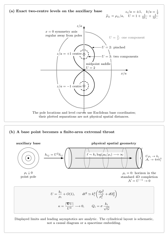
For the selected equal collinear example with centres at $z/a=\pm1$ and $k/a=1/2$, the exact meridional auxiliary-base level-set cross-sections $U=3/2$, $2$, and $3$ respectively enclose both poles, pinch at the midpoint saddle, and split into two components. These are not proper-distance contours. Near any positive pole, $U\sim k_i/\rho_i$: the lapse vanishes and physical radial distance diverges logarithmically, while $U\rho_i\to k_i$ and the limiting sphere has area $4\pi k_i^2$; the signed charge is $Q_i=\sigma k_i/\sqrt G$ and $\kappa_i=0$. The upper curves and equations are exact; the lower throat layout is schematic, and the horizon label invokes the standard four-dimensional completion rather than following from the local picture alone.

One centre gives extremal Reissner–Nordström

For $N=1$, write $k=GM$ and $\rho=\lvert\mathbf x\rvert$. The areal radius

$$R=U\rho=\rho+k$$

maps the original domain $\rho>0$ only to the exterior $R>k$. In these coordinates,

$$\begin{aligned} ds^2&=-\left(1-\frac{k}{R}\right)^2dt^2 +\left(1-\frac{k}{R}\right)^{-2}dR^2 +R^2d\Omega_2^2,\\ A&=-\frac{\sigma k}{\sqrt G\,R}\,dt, \qquad F=\frac{\sigma k}{\sqrt G\,R^2}\,dR\wedge dt. \end{aligned}$$

Comparing with the general Reissner–Nordström lapse

$$f(R)=1-\frac{2GM}{R}+\frac{GQ^2}{R^2}$$

gives $Q=\sigma\sqrt G\,M$ and $f=(1-k/R)^2$. This recovers the sign as well as the magnitude of the charge.

The diagonal coordinate singularity at $R=k$ is removable. Define an advanced coordinate by

$$dv=dt+\frac{dR}{f(R)}.$$

Then

$$ds^2=-f\,dv^2+2\,dv\,dR+R^2d\Omega_2^2, \qquad F=\frac{Q}{R^2}\,dR\wedge dv.$$

The $(v,R)$ metric block has determinant $-1$, and both the metric and the field are finite at $R=k$. The new chart genuinely crosses one selected horizon branch; it is not merely a relabeling of the original $\rho>0$ exterior.

Why arbitrary positions remain in balance

The positions $\mathbf x_i$ never entered the field-equation reduction except through a harmonic superposition. Once all $k_i>0$ and one common $\sigma$ are chosen, every set of distinct locations gives a smooth source-free electrovac solution on the punctured exterior. This is the exact nonlinear content of balance.

A weak-field calculation is a useful check, but not the proof. For two centres separated by $d$,

$$F_{\mathrm{grav}}=\frac{GM_iM_j}{d^2}, \qquad F_{\mathrm{elec}}=\frac{Q_iQ_j}{d^2} =\frac{GM_iM_j}{d^2}.$$

The forces oppose one another because the charges have the same sign. Opposite signs make the electric and gravitational attractions point the same way and are incompatible with this static positive-pole ansatz.

What about a conical strut? Generic non-collinear configurations have no common symmetry axis, so an “axis segment between every pair” is not even defined. The general statement is that the metric and Maxwell field are smooth electrovac away from the poles. In the collinear axisymmetric subclass, one can also check elementary flatness directly. In cylindrical base coordinates,

$$h=U^2\left(d\varpi^2+dz^2+\varpi^2d\phi^2\right), \qquad \phi\sim\phi+2\pi.$$

At a regular axis point away from a pole, $U(\varpi,z)=U_0(z)+O(\varpi^2)$. Therefore

$$\frac{\text{proper circumference}} {\text{proper radius}} = \frac{2\pi U\varpi} {\int_0^\varpi U(\varpi',z)\,d\varpi'} \longrightarrow2\pi.$$

No conical deficit or excess is present. Conformal flatness alone is not the argument; the smooth even expansion of $U$ and the $2\pi$ angular period are essential.

Exterior, analytic crossing, and global choices

For positive residues, $U>0$ everywhere on the punctured base. The static exterior is thus a connected, asymptotically flat, source-free domain with one normalized infinity and $N$ infinite throat ends. The area, surface-gravity, invariant, and near-horizon calculations identify each end as a regular local extremal-horizon candidate.

Global event-horizon language needs an extension. Hartle and Hawking constructed analytic coordinates across the positive centres and showed that the standard four-dimensional family can be interpreted as several charged black holes in equilibrium Hartle and Hawking 1972, § II, pp. 90–94, especially Eqs. (2.9)–(2.16) and Figs. 1–4, Open PDF. Bičák gives a compact modern summary, including the individual horizon areas and bounded four-dimensional extension statement, in Bičák 2000, § 5, pp. 53–54, Eqs. (30)–(33), Open PDF.

Three qualifications matter.

1. The local limits above do not by themselves identify an event horizon, because an event horizon is defined relative to the causal future and the chosen asymptotic completion.
2. Crossing a horizon does not force one unique maximal global gluing. The analytic blocks may be continued and joined in more than one way; on continued sheets a surface where the continued harmonic factor vanishes is a genuine curvature singularity, not another harmless base pole.
3. Exact equilibrium proves neither dynamical stability nor formation from regular collapse data. Those are perturbative and evolutionary questions.

The scope here is therefore the standard time-unwrapped asymptotically flat exterior, its regular local horizon crossings, and the classic four-dimensional multi-black-hole interpretation—not a claim that the exterior data select every global identification.

Controlled limits and failure modes

The same formulas make good and bad limits easy to distinguish.

Operation	Data held fixed	Result	What it teaches
Flat limit	Fixed $\mathbf x$ away from all centres; every $k_i\to0$	$U\to1$, $F\to0$, and $g\to\eta$	Gravity and electromagnetism disappear together.
Remove one centre	Fixed remaining positions and residues; $k_j\to0$	The $j$th harmonic term and its charge vanish	Centre removal is continuous away from the removed point.
Single-centre limit	Keep one $k_i>0$ and remove the others	Extremal Reissner–Nordström exterior	The multi-centre normalization matches the spherical benchmark.
Coalesce centres	$\mathbf x_i=\mathbf x_0+\varepsilon\boldsymbol\lambda_i$, fixed $\mathbf x\ne\mathbf x_0$, then $\varepsilon\to0$	$U\to1+(\sum_i k_i)/\lvert\mathbf x-\mathbf x_0\rvert$	Convergence is smooth on compact sets away from $\mathbf x_0$, but $N$ horizon components become one; this is not global fixed-topology convergence.
Negative residue	For one centre, $U=1-k/\rho$ with $k>0$	$U=0$ at $\rho=k$ and $R_{\mu\nu}R^{\mu\nu}=4k^4/(\rho-k)^8$ diverges	A zero of $U$ is a curvature singularity, not a regular extremal horizon.
Opposite charge sign	Keep positive masses but reverse one electric charge	The shared-potential Einstein–Maxwell cancellation fails	Common sign is part of the exact solution, not a cosmetic convention.

More general harmonic functions may be useful locally, but multipoles, nonconstant asymptotic terms, or sign changes can destroy asymptotic flatness or introduce naked singularities. The displayed family is purely electric. A single electromagnetic duality rotation produces aligned dyonic representatives, but the same duality angle must be used for every centre if the common-potential balance is to be preserved.

Common pitfalls

Treating $\rho_i=0$ as a material point charge. It is a point only in the auxiliary Euclidean base. Positive residues give finite-area, infinite-distance horizon ends after the geometric and extension checks.

Calling every surface with $g_{tt}=0$ an event horizon. Vanishing lapse is local information. Smooth horizon crossing and the causal completion are separate requirements.

Explaining balance by conformal flatness. The exact balance follows from the coupled field equations reducing to one harmonic function. Elementary flatness supplies a separate no-strut check only where an axis exists.

Allowing independent charge signs. One global $\sigma$ fixes every $Q_i$. Changing a single sign while keeping the same positive-mass harmonic metric no longer solves the coupled equations.

Exercises

1. Derive the Maxwell reduction

Starting from the conformastatic ansatz, compute $F_{it}$, $F^{it}$, and $\partial_i(\sqrt{-g}F^{it})$.

Solution

Because $A_t=\sigma(U^{-1}-1)/\sqrt G$,

$$F_{it}=\partial_iA_t =-\frac{\sigma}{\sqrt G}U^{-2}\partial_iU.$$

The inverse metric has $g^{tt}=-U^2$ and $g^{ij}=U^{-2}\delta^{ij}$, so

$$F^{it} =g^{ij}g^{tt}F_{jt} =\frac{\sigma}{\sqrt G}U^{-2}\delta^{ij}\partial_jU.$$

Since $\sqrt{-g}=U^2$,

$$\partial_i(\sqrt{-g}F^{it}) =\frac{\sigma}{\sqrt G} \partial_i(\delta^{ij}\partial_jU) =\frac{\sigma}{\sqrt G}\nabla^2U.$$

Thus the source-free Maxwell equation is precisely the flat Laplace equation away from the poles.

2. Recover the signed one-centre charge

For $U=1+k/\rho$, transform both the metric and potential with $R=\rho+k$, and compare with general Reissner–Nordström rather than assuming extremality.

Solution

Since $U=R/(R-k)$ and $d\rho=dR$,

$$ds^2 =-\left(1-\frac{k}{R}\right)^2dt^2 +\left(1-\frac{k}{R}\right)^{-2}dR^2 +R^2d\Omega_2^2.$$

Also,

$$A =\frac{\sigma}{\sqrt G} \left(\frac{R-k}{R}-1\right)dt =-\frac{\sigma k}{\sqrt G\,R}\,dt.$$

The standard gauge is $A=-Q\,dt/R$, so $Q=\sigma k/\sqrt G$. Comparing

$$\left(1-\frac{k}{R}\right)^2 =1-\frac{2k}{R}+\frac{k^2}{R^2}$$

with $1-2GM/R+GQ^2/R^2$ gives $k=GM$ and $Q=\sigma\sqrt G\,M$. The original coordinate range is $R>k$; the advanced chart is needed to cross $R=k$.

3. Check area, distance, and degeneracy

Assume $U=k/\rho+H$ with $H=O(1)$. Show that the limiting sphere area is finite, the proper radial distance diverges, and $\kappa=0$.

Solution

On $\rho=\text{constant}$ the exact induced metric and area are

$$\gamma_{AB}=(U\rho)^2\Omega_{AB}, \qquad \mathcal A(\rho)=\int_{S^2}(U\rho)^2\,d\Omega.$$

Although $H$ may depend on angle, $U\rho=k+O(\rho)$ uniformly. Thus $\gamma_{AB}\to k^2\Omega_{AB}$ and $\mathcal A\to4\pi k^2$. Along a radial line,

$$\int_\rho^{\rho_0}U\,d\rho' =k\log\!\frac{\rho_0}{\rho}+O(1),$$

so the static slice has an infinite throat. Finally, $\lvert\boldsymbol\nabla U\rvert=k/\rho^2+O(1)$ and $U^3=k^3/\rho^3+O(\rho^{-2})$, giving

$$\kappa =\lim_{\rho\to0}\frac{\lvert\boldsymbol\nabla U\rvert}{U^3} =\lim_{\rho\to0}\frac{\rho}{k^2}=0.$$

Finite area, infinite distance, and zero surface gravity are mutually consistent signatures of an extremal throat.

4. Verify elementary flatness

For collinear centres, prove that a regular portion of the symmetry axis has no conical deficit.

Solution

Smooth axisymmetry gives $U(\varpi,z)=U_0(z)+O(\varpi^2)$ away from poles. A small circle has proper circumference

$$C=2\pi\sqrt{h_{\phi\phi}}=2\pi U\varpi =2\pi U_0\varpi+O(\varpi^3).$$

Its proper radius is

$$L=\int_0^\varpi\sqrt{h_{\varpi\varpi}}\,d\varpi' =\int_0^\varpi U(\varpi',z)\,d\varpi' =U_0\varpi+O(\varpi^3).$$

Therefore $C/L\to2\pi$. This calculation uses smoothness and the standard angular period; conformal flatness by itself would not fix the ratio.

5. Separate coalescence from a negative residue

(a) Let $\mathbf x_i=\mathbf x_0+\varepsilon\boldsymbol\lambda_i$. Find the pointwise limit of $U$ at fixed $\mathbf x\ne\mathbf x_0$. (b) For $U=1-k/\rho$, locate the zero and evaluate the Ricci-square behavior there.

Solution

For fixed $\mathbf x\ne\mathbf x_0$,

$$\frac{1}{\lvert\mathbf x-\mathbf x_i\rvert} \longrightarrow \frac{1}{\lvert\mathbf x-\mathbf x_0\rvert},$$

so

$$U\longrightarrow 1+\frac{\sum_i k_i}{\lvert\mathbf x-\mathbf x_0\rvert}.$$

The convergence is smooth on compact sets excluding $\mathbf x_0$, but it cannot preserve the number of horizon components because several poles become one.

For the negative residue, $U=0$ at $\rho=k$. Since $\lvert\boldsymbol\nabla U\rvert^2=k^2/\rho^4$,

$$R_{\mu\nu}R^{\mu\nu} =4U^{-8} \left(\lvert\boldsymbol\nabla U\rvert^2\right)^2 =\frac{4k^4}{(\rho-k)^8}.$$

The zero surface is a genuine curvature singularity. It is qualitatively different from the finite-invariant positive-pole horizon.

6. Diagnose the midpoint saddle in the figure

For the equal two-centre example in the figure, use the signed meridional coordinate $\widehat x=x/a$ and $\widehat z=z/a$, with

$$U=1+\frac{1}{2\widehat\rho_+} +\frac{1}{2\widehat\rho_-}, \qquad \widehat\rho_\pm =\sqrt{\widehat x^2+(\widehat z\mp1)^2}.$$

Evaluate $U$ and its gradient at the midpoint, compute the Hessian in the $(\widehat x,\widehat z)$ meridional plane, and explain the topology change shown by the level curves.

Solution

At $(\widehat x,\widehat z)=(0,0)$, both normalized distances equal one, so $U=2$. The contributions linear in $\widehat z$ cancel between the two centres, while reflection across the symmetry axis makes the first $\widehat x$ derivative vanish. Thus $\boldsymbol\nabla U=0$.

Expanding to quadratic order gives

$$U =2-\frac12\widehat x^2+\widehat z^2 +O\!\left((\widehat x^2+\widehat z^2)^{3/2}\right).$$

Therefore

$$\left.\operatorname{Hess}U\right|_{(0,0)} =\begin{pmatrix}-1&0\\[2pt]0&2\end{pmatrix}.$$

Its opposite-sign eigenvalues make the midpoint a saddle. The critical level $U=2$ pinches there; the lower level $U=3/2$ passes around both centres as one component, while the higher level $U=3$ has two components, one around each centre, exactly as the upper panel shows.

The next chapter develops the symmetry reduction behind rotating equilibrium geometries: Stationary and Axisymmetric Spacetimes.

References

• Bičák, Jiří. “Selected Solutions of Einstein’s Field Equations: Their Role in General Relativity and Astrophysics.” In Einstein’s Field Equations and Their Physical Implications, edited by Bernd G. Schmidt, Lecture Notes in Physics 540, 1–126. Berlin: Springer, 2000. DOI: 10.1007/3-540-46580-4_1. arXiv:gr-qc/0004016v1. Open PDF.
• Hartle, James B., and Stephen W. Hawking. “Solutions of the Einstein–Maxwell Equations with Many Black Holes.” Communications in Mathematical Physics 26, no. 2 (1972): 87–101. DOI: 10.1007/BF01645696. Open PDF.
• Majumdar, Sudhansu Datta. “A Class of Exact Solutions of Einstein’s Field Equations.” Physical Review 72, no. 5 (1947): 390–398. DOI: 10.1103/PhysRev.72.390.