What does it mean for the universe to expand?

Cosmic expansion means that the average separation of widely spaced, freely moving galaxies changes with time. In the expanding-universe description, larger separations grow by larger amounts over the same short interval.

This is a statement about the universe on large scales. It does not mean that rulers, people, planets, and galaxies all stretch together. Nor does it require galaxies to be flying away from one special explosion site into a surrounding empty space.

The scale factor compares separations at different times

Imagine marking several positions that follow the large-scale expansion. Such positions are called comoving. A number called the scale factor tells us how their separations change: if it grows by a factor of 1.5, each corresponding separation grows by that factor.

The two grids below show the same labeled positions at two times. Follow A–B and A–C rather than looking for a privileged center.

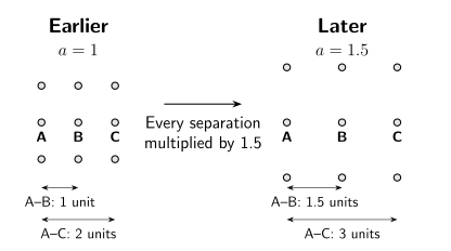
An idealized comoving pattern expands by the same factor about any chosen reference point. Distances use arbitrary units; the diagram shows a finite patch, not the edge or center of the universe. Galaxy symbols keep the same size to distinguish large-scale separations from the sizes of bound systems. This is a model illustration, not a galaxy survey.

Open full-size diagram

Pair	Earlier separation	Later separation	Increase
A–B	1 unit	1.5 units	0.5 unit
A–C	2 units	3 units	1 unit

The more distant pair has a larger increase, but the fractional increase is the same: 50 percent. Choose B as the reference instead of A and the same rule holds.

Actual galaxies also have motions caused by local gravity. Nearby galaxies can approach one another, and bound groups do not simply follow this grid. Expansion is the large-scale background against which those additional motions occur.

Redshift connects traveling light to that changing scale

Astronomers recognize patterns of spectral lines and compare their wavelengths with laboratory measurements. The fractional increase in wavelength is the redshift, written $z$.

For light traveling between comoving observers in a homogeneous expanding model, the wavelength grows by the same factor as the scale factor between emission and reception. A wavelength received at twice its emitted value has $z=1$; this corresponds to a scale factor twice as large at reception.

That relationship concerns cosmological redshift. Local motions and gravity can also shift wavelengths, so an observed redshift must be interpreted in context (Carroll 2014, §8.5, pp. 344–346).

It is tempting to turn every redshift into a speed by multiplying by the speed of light. The approximation $v\simeq cz$ is useful at small redshift, but it is not a universal rule for distant galaxies. A cosmological recession rate compares distances at the same cosmic time; the spectrum arriving now carries information from the past.

The nearby Hubble relation has a limited job

At sufficiently small redshift, the distance–redshift relation is approximately linear:

$$cz\simeq H_0D.$$

Here $c$ is light speed, $H_0$ is today’s Hubble constant, and $D$ is a nearby distance, where the usual cosmological distance definitions approximately agree. Local motions can add appreciable scatter (Hogg 1999, §3, Eq. (10)).

As an example, choose $H_0=70$ kilometers per second per megaparsec. One megaparsec, or Mpc, is a million parsecs. A model galaxy at 100 Mpc has $H_0D=7{,}000$ km/s and a small-redshift estimate of about 0.023. These are illustrative parameters, not a claim to settle the measured value of $H_0$.

Now add a hypothetical 300 km/s motion along the line of sight. It is a modest fraction of 7,000 km/s, but a large fraction of the model recession rate of 700 km/s at 10 Mpc. This helps explain why the nearest galaxies need special care rather than automatically giving the cleanest expansion measurement.

“How far away?” needs a distance definition

Looking far away means looking back in time. The source emitted the light when the universe had a different scale factor, so one distance number cannot serve every purpose.

• Proper distance at a chosen cosmic time describes a spatial separation in the model at that time. Today’s value is not read directly from a photograph.
• Comoving distance removes the scale-factor growth, making positions that follow the expansion retain fixed separations in those coordinates.
• Luminosity distance is defined by comparing a source’s luminosity with its received, frequency-integrated flux.
• Angular-diameter distance compares a source’s physical transverse size at emission with its observed angular size.

These quantities agree approximately nearby but can differ substantially at large redshift (Hogg 1999, §§4, 6, and 7).

Likewise, multiplying light-travel time by $c$ does not generally give today’s proper distance. The light traveled while the intervening geometry changed. A quoted distance is most useful when its definition and assumed cosmological model accompany it.

Try the mathematics: expansion rate and redshift

Preparation: algebra and ratios for redshift; derivatives for the instantaneous expansion rate.

Choose a dimensionless scale factor $a(t)$ and let $\chi$ be a fixed comoving radial separation, with units of length. The proper separation is

$$D(t)=a(t)\chi, \qquad \frac{dD}{dt}=H(t)D(t), \qquad H(t)=\frac{\dot a(t)}{a(t)}.$$

A dot denotes a time derivative. This is the same-time kinematic relation in the homogeneous model. It does not make $cz$ an exact recession speed at arbitrary redshift.

For photons traveling between comoving observers,

$$1+z=\frac{\lambda_{\rm observed}}{\lambda_{\rm emitted}} =\frac{a_{\rm observed}}{a_{\rm emitted}}.$$

If today’s scale factor is one, light with cosmological redshift three was emitted when it was one-quarter. This gives a relative scale, not an age by itself: converting scale factor to time requires an expansion history.

Optional deeper reading. Cosmological Redshift derives the relation between measured frequency and the scale factor, including its assumptions. Preparation: calculus, spacetime metrics, and null geodesics.

Predict what changes when you change the observer

In the figure, A–B grows from one to 1.5 units. From B, the separation to C does the same. Does choosing B make B a new physical center? Would a locally approaching pair of galaxies disprove large-scale expansion?

Answer and transfer

Choosing B changes the reference point, not the pattern. Every pair still grows by 50 percent. No labeled position is a special expansion center.

A nearby approaching pair does not by itself disprove the large-scale description: the pair may be bound or have local motions that dominate its separation change. The model must be tested on appropriate scales and against many measurements.

Finally, the two snapshots alone do not establish whether expansion is accelerating. That requires evidence that the rate at which the scale factor grows is itself increasing. The next question is how distance measurements test dark energy.

For educators

Preparation and objective. The main activity needs multiplication and ratios. Students should distinguish equal fractional expansion from equal added distances, and separate expansion from local motion.

Short activity, about 10 minutes. Choose different grid points as observers and compare three pair separations. Expected answer: every comoving separation grows by 50 percent in the illustrated snapshots, although larger separations gain more length. The chosen observer does not become a physical center.

Longer extension, about 30 minutes. Add an independent motion to one point and identify which simple grid rule it violates. Use the 10 and 100 Mpc examples to compare a 300 km/s local motion with the model recession rates: about 43 percent and 4.3 percent, respectively. Discuss why a nearby approaching pair does not disprove large-scale expansion.

Misconception to discuss. “Everything, including rulers, must expand.” Bound systems do not simply track the scale factor. Likewise, the drawing’s paper edge is not an edge of space, and two snapshots alone do not establish acceleration; the explained task above gives the reason.

References

• Carroll, S. M. (2014). Spacetime and Geometry: An Introduction to General Relativity. Pearson New International Edition, §§8.3 and 8.5. Author’s book page.
• Hogg, D. W. (1999; version 4, 16 December 2000). “Distance Measures in Cosmology.” arXiv:astro-ph/9905116. Manuscript record; author text hosted by NED.