What can starlight tell us?

A point of starlight contains more information than its brightness suggests. Spread that light by wavelength and measure how much arrives in each small interval: the result is a spectrum. Its broad shape, its narrow features, and shifts in those features provide different clues about the source and the material between it and us.

Predict first. Two spectra have the same distinctive pattern of dips, but the wavelength scale of one pattern is slightly stretched. Is a different mixture of elements the only explanation?

A spectrum is a measurement

Wavelength measures the spacing between successive crests of a light wave. Visible red light has a longer wavelength than visible blue light. Infrared, ultraviolet, radio waves, and X-rays also belong to the electromagnetic spectrum, even though our eyes cannot see them.

A spectrograph separates incoming light by wavelength. A detector then records the signal. Astronomers calibrate the detector response and wavelength scale to turn that signal into useful measurements. A spectrum can be shown as coloured bands, but a graph of measured light against wavelength usually makes small features easier to compare.

The panels below separate a smooth continuum, a pattern of lines, and a common fractional wavelength shift. Compare absorption and emission at the same wavelengths. The invented line positions are teaching examples, not an identification of a real element.

1. Continuous light

A smooth background supplies light across this wavelength interval.

Wavelength in nanometres → · vertical: relative light intensity

A real continuum need not be flat. Its broad shape helps constrain temperature, once other effects such as dust are accounted for.

2. A pattern of lines

Match the wavelengths of several features. Dips and peaks can mark the same transitions.

Absorption: dips

Emission: peaks

Same wavelength axis in both views · vertical heights are illustrative

These invented line positions do not identify an element. Real line strengths depend on physical conditions as well as abundance.

3. The whole pattern shifts

Multiply every wavelength by 1.0002. The increases differ, but the fractional change is the same.

Reference 400.00 nm

Shifted 400.08 nm
Increase 0.08 nm

Reference 500.00 nm

Shifted 500.10 nm
Increase 0.10 nm

Reference 650.00 nm

Shifted 650.13 nm
Increase 0.13 nm

Each increase divided by its reference wavelength is 0.0002. These are the article's numerical examples, not observed spectral lines. No line-height change is implied.

Different features answer different questions: continuum shape, line pattern, and a common fractional wavelength shift. The curves are original teaching schematics; intensities and triangular profiles are not physical predictions. The numbers in the final panel preserve the stated wavelength ratio.

View the continuous, absorption, and emission patterns together

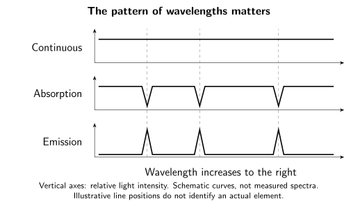
Spectral features connect light to matter. Horizontal axes increase in wavelength; vertical axes show relative light intensity. These are schematic patterns with invented line positions and no measured wavelength scale. The flat continuum simplifies a small spectral region; real continua need not be flat.

Open full-size diagram

Three clues in the same light

The broad shape helps estimate temperature. Hot, dense sources emit across a broad range of wavelengths. In a simple thermal model, raising the temperature shifts the peak of the energy spectrum toward shorter wavelengths. A hot stellar surface therefore tends to look bluer than a cooler one. Astronomers compare calibrated measurements with atmosphere models because interstellar dust and other effects can alter the light on its journey. Fraknoi, Morrison, and Wolff 2022, § 5.2, “Radiation Laws”

Narrow lines help identify matter. Atoms and molecules exchange light at characteristic wavelengths. Gas can remove some wavelengths from light passing through it, producing absorption dips. Excited gas can also emit particular wavelengths, producing peaks. A pattern of several matching features is more persuasive than one isolated coincidence. The strength of a line depends on physical conditions as well as abundance; a weak or missing line does not automatically mean an element is absent. NASA, ESA, CSA, and STScI 2021, “Types of Spectra,” absorption and emission descriptions

A shifted pattern helps measure motion. Once we identify a set of lines, we can compare their measured wavelengths with laboratory values. Motion away from us shifts the pattern toward longer wavelengths; motion toward us shifts it toward shorter wavelengths. The pattern in the opening question could therefore come from similar material moving differently along our line of sight. We compare fractional shifts, not simply a fixed number of pixels on a picture. Fraknoi, Morrison, and Wolff 2022, § 5.6, “The Doppler Effect”

Measured feature	A possible inference	What else matters?
Broad distribution over wavelength	Surface temperature	Dust, calibration, and an appropriate emission model
Identified absorption or emission lines	Atoms or molecules in the emitting or absorbing material	Temperature, density, ionization, and blended lines
Common fractional shift of identified lines	Motion along the line of sight	Observer motion and other causes of redshift

From a line shift to a speed

Consider an invented example: a laboratory line at 500.0 nanometres appears at 500.1 nanometres. The measured wavelength is longer by 0.1 nanometres. If the shift is caused by slow relative motion, it corresponds to recession at about 60 kilometres per second.

One line might be misidentified or blended with another. Compare three instead. Each row below has the same fractional wavelength increase, although the differences in nanometres are unequal.

Laboratory wavelength	Observed wavelength	Increase divided by laboratory wavelength
400.00 nm	400.08 nm	0.08/400 = 0.0002
500.00 nm	500.10 nm	0.10/500 = 0.0002
650.00 nm	650.13 nm	0.13/650 = 0.0002

These are teaching values, not measured lines from an identified element. Their common ratio is what makes them consistent with one Doppler shift. Simply adding 0.1 nm to every wavelength would give different fractional shifts and would not reproduce this pattern.

Show the math: the slow-motion Doppler approximation

For radial speed much smaller than the speed of light, and with other shifts removed,

$$\frac{\lambda_{\rm observed}-\lambda_{\rm rest}}{\lambda_{\rm rest}} \approx\frac{v_r}{c}.$$

Here $v_r$ is positive for recession. The example has fractional shift $0.1/500=0.0002$. Multiplying by $c\approx300{,}000\ {\rm km\,s^{-1}}$ gives $v_r\approx60\ {\rm km\,s^{-1}}$. The units are consistent: a ratio of wavelengths is dimensionless.

This measures one component of motion. A star can also move sideways. Large speeds require relativistic treatment. A measured redshift can also include gravitational effects or cosmological expansion, so its cause must be established before applying this relative-motion formula.

Repeat the measurement, then test the explanation

The telescope moves as Earth rotates and orbits the Sun. Astronomers account for that observer motion when comparing stellar velocities at different times. They also calibrate the wavelength scale against stable references: an instrument drift can imitate a line shift. For example, the HARPS instrument uses simultaneous reference spectra to track changes, and its reduced one-dimensional spectra use a reference frame tied to the Solar System’s centre of mass. ESO n.d., HARPS science modes, § Simultaneous Thorium Reference Method; Mascetti 2024, HARPS data products, § S1D

A repeating change from recession to approach can reveal orbital motion around a shared centre of mass. That connects spectroscopy to weighing stars and finding planets. It is still a hypothesis to test. Changes on the star’s surface can distort line shapes and mimic a small velocity signal; astronomers compare other activity indicators and repeated observations before assigning an orbit. ESO n.d., “HARPS,” stellar-activity discussion

Try a red-looking star

A star looks red in a photograph. Is that enough to claim that it is rapidly moving away?

Answer

No. Its surface may be relatively cool, dust may have removed more of the blue light, or the picture may use an assigned colour scheme. A Doppler measurement compares identified line wavelengths with reference wavelengths. Broad colour and a precisely shifted spectral pattern answer different questions.

For classrooms and clubs

Preparation: reading axes; ratios help with the numerical activity. Objective: distinguish a measured shift from its possible explanations. In 15 minutes, compare the three rows of the wavelength table. Learners should recover the same fractional shift from unequal wavelength differences; adding an unrelated line need not change the identification of the matching set. The table supports a text-only comparison. No direct viewing of the Sun, laser, or bright lamp is needed.

For a longer extension, let the same rest wavelengths be multiplied by 0.9998 at a second epoch. The simple Doppler model changes from about 60 km/s recession to about 60 km/s approach. Ask what must be checked before claiming a companion: observer motion, wavelength calibration, stellar variability, and further repeat measurements. The common misconception is that a red-looking photograph measures recession; the solved question distinguishes broad colour from identified line shifts.

Next, see why telescopes need both collecting area and sharpness, or use stellar properties to explore the H–R diagram.

References

• European Southern Observatory. “HARPS.” n.d. Instrument and stellar-activity discussion. Accessed September 27, 2026.
• European Southern Observatory. “HARPS Science Modes.” n.d. Simultaneous Thorium Reference Method. Accessed September 27, 2026.
• Fraknoi, Andrew, David Morrison, and Sidney Wolff. Astronomy 2e. Houston: OpenStax, 2022. § 5.2, “The Electromagnetic Spectrum”; § 5.6, “The Doppler Effect”.
• Mascetti, Laura. “HARPS – How to Get the Pipeline Generated Files: CCF, S1D, E2DS, BIS, INT, GUIDE.” ESO Operations Helpdesk, updated May 15, 2024. Data-product descriptions.
• NASA, ESA, CSA, and Space Telescope Science Institute. “Types of Spectra: Continuous, Emission, and Absorption.” NASA Science, July 2, 2021. Explanatory descriptions.

Further reading

For an optional extension beyond the low-speed Doppler approximation, read Photons, Doppler Shift, and Aberration. It compares frequencies and directions measured by different observers. Preparation: special relativity, four-vectors, and linear algebra.